A&A 403, 443-448 (2003)
DOI: 10.1051/0004-6361:20030328
A. Mészáros - J. Stocek
Astronomical Institute of the Charles University, V Holesovickách 2, 180 00 Prague 8, Czech Republic
Received 15 March 2002 / Accepted 28 February 2003
Abstract
The gamma-ray bursts detected by the BATSE instrument may be separated
into "short", "intermediate" and "long" subgroups. Previous
statistical tests found an anisotropic sky-distribution on large
angular scales for the intermediate subgroup, and probably also
for the short subgroup. In this article the description and the
results of a further statistical test - namely the nearest
neighbour analysis - are given. Surprisingly, this test gives an
anisotropy for the long subgroup on small angular scales. The
discussion of this result suggests that this anisotropy may be
real.
Key words: gamma-rays: bursts - cosmology: miscellaneous
The separation of the gamma-ray bursts (hereafter GRBs) - detected
by the BATSE instrument (Meegan et al. 2000) - into subgroups is done
(Kouveliotou et al. 1993; Horváth 1998;
Mukherjee et al. 1998) with respect to T90,
the duration during which 90% of the radiation of a burst is
measured. Bursts are either short (
![]() s), or
intermediate (
s), or
intermediate (
![]() ), or long (
T90
> 10 s). Nowadays it is practically sure that the long and short
subgroups are different phenomena (Norris et al. 2001; Horváth et al. 2001).
The situation concerning the intermediate subgroup is unclear;
some authors query even the reality of this subgroup itself
(Hakkila et al. 2000). From the afterglow data the cosmological origin is
directly confirmed for the long bursts only. They are usually at
high redshifts. For the short and intermediate GRBs there is only
indirect evidence for a cosmological origin, and concrete
redshifts are unknown (for a survey of these questions see
Mészáros P. 2001).
), or long (
T90
> 10 s). Nowadays it is practically sure that the long and short
subgroups are different phenomena (Norris et al. 2001; Horváth et al. 2001).
The situation concerning the intermediate subgroup is unclear;
some authors query even the reality of this subgroup itself
(Hakkila et al. 2000). From the afterglow data the cosmological origin is
directly confirmed for the long bursts only. They are usually at
high redshifts. For the short and intermediate GRBs there is only
indirect evidence for a cosmological origin, and concrete
redshifts are unknown (for a survey of these questions see
Mészáros P. 2001).
During the last years one of the authors together with various collaborators provided several statistical tests verifying the isotropy in the angular distribution of GRBs. These tests were based on the binomial distribution (Mészáros A. 1997; Balázs et al. 1998; Balázs et al. 1999), on spherical harmonics (Mészáros A. et al. 2000a), on the counts-in-cells method (Mészáros A. et al. 2000b), on the two-point angular correlation function (Mészáros A. et al. 2000c), and on multifractal methods (Vavrek et al. 2001). These tests (for a summary see Mészáros A. et al. 2001) give an anisotropy for the intermediate subgroup. The short subgroup also seems to be distributed anisotropically; nevertheless, there are only a few tests that reject isotropy at a high enough confidence level. The long subgroup seems to be distributed isotropically; here only the test based on the two-point angular correlation function rejects the null hypothesis of isotropy (Mészáros A. et al. 2000c). Recently and fully independently these results were confirmed by Litvin et al. (2001).
In this paper we present the results of a new test; namely of the nearest neighbour analysis (hereafter NNA). This test (Scott & Tout 1989) is a standard statistical test, and - as far as known - has not been used yet for GRBs.
The paper is organized as follows. In Sect. 2 the method is described. Section 3 compares this method with other methods. Section 4 presents the results of the test. Section 5 discusses and summarizes the conclusions of the paper.
NNA is a standard statistical test, which compares the actual angular distances among the objects on the surface of a sphere having unit radius with the theoretical angular distances in a randomly and isotropically distributed sample.
The theory of NNA was formulated by Scott & Tout (1989). Here this theory is only recapitulated and specified for the sky distribution of GRBs.
Let there be N objects on the sky, which are distributed
randomly. N should be ![]() 2; for our purpose we may assume
2; for our purpose we may assume ![]() .
We arbitrarily choose one object ("first object"). At an
angular distance
.
We arbitrarily choose one object ("first object"). At an
angular distance ![]() (
(
![]() )
from the first
object we define an infinitesimal belt with thickness d
)
from the first
object we define an infinitesimal belt with thickness d![]() .
This belt is defined by the distance interval
.
This belt is defined by the distance interval
![]() .
The probability of having (L-1) objects at the
distance
.
The probability of having (L-1) objects at the
distance ![]()
![]() ,
and one object in the infinitesimal belt is
given by
,
and one object in the infinitesimal belt is
given by
| |
(1) |
The integral probability
![]() defines the probability that there are L and
exactly L objects in the neighbourhood of the first object; the
neighbourhood is defined by the distances
defines the probability that there are L and
exactly L objects in the neighbourhood of the first object; the
neighbourhood is defined by the distances
![]() .
.
![]() ,
as it should be. For L=1 and L=2 one
obtains
,
as it should be. For L=1 and L=2 one
obtains
 |
(2) |
| (3) |
If the integral probabilities for different L are given by these analytical formulas, we can use them as theoretical cumulative probability distributions. The standard Kolmogorov-Smirnov test can be used to compare them with the measured empirical cumulative distributions (Press et al. 1992; Chap. 14.3).
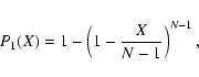
The test for L=1 should be done as follows. The theoretical
function P1(X) is defined for
![]() and is
monotonously increasing from 0 to 1. The measured (N-1)first nearest neighbour distances are sorted into increasing
sequence. Then, for any distance in this sequence, one obtains a
value X, and at this value the empirical cumulative distribution
function is increased by the value
(N-1)-1. Hence the
empirical cumulative function also runs from 0 to 1 for the
same range of X. The maximal absolute value D between the two
different cumulative distribution functions defines the
significance level for given (N-1) (Press et al. 1992, Chap. 14.3).
and is
monotonously increasing from 0 to 1. The measured (N-1)first nearest neighbour distances are sorted into increasing
sequence. Then, for any distance in this sequence, one obtains a
value X, and at this value the empirical cumulative distribution
function is increased by the value
(N-1)-1. Hence the
empirical cumulative function also runs from 0 to 1 for the
same range of X. The maximal absolute value D between the two
different cumulative distribution functions defines the
significance level for given (N-1) (Press et al. 1992, Chap. 14.3).
One can do (N-1) tests, because the test may be done for any allowed L. For any L the theoretical cumulative function can be calculated and is an analytical function. The (N-1) Lth nearest neighbour measured angular distances can also be obtained from the positions of objects.
However, one does not need to provide all possible (N-1) tests for one sample. Let us assume that the test is made for L=1, then for L=2, ..., then for L = (N-1). If one assumes that the null hypothesis is true, viz. that the objects are distributed randomly on the surface of the sphere, then no test should reject this hypothesis. Nevertheless, it is unlikely that going to bigger and bigger L will give any new result. This may be seen as follows.
There are N(N-1)/2 distances among the observed N objects. But
only (2N-3) distances are independent. (N objects on the
sphere are defined by 2N coordinates (any object is defined by
two spherical angles, e.g. by ![]() and
and ![]() ).
Nevertheless, one object may be taken - without loss of generality
- at the pole (i.e. one may have
).
Nevertheless, one object may be taken - without loss of generality
- at the pole (i.e. one may have
![]() for this "first
object"). A second arbitrary object may still be at
for this "first
object"). A second arbitrary object may still be at
![]() .
There are (N-1) independent distances known immediately: they
are the
.
There are (N-1) independent distances known immediately: they
are the ![]() coordinates of (N-1) objects giving the
distances from the first object. There are a further (N-2)independent distances from the second object. They can be
calculated if the
coordinates of (N-1) objects giving the
distances from the first object. There are a further (N-2)independent distances from the second object. They can be
calculated if the ![]() coordinates are known. Then any
further distances can be calculated from these (2N-3) independent distances.)
coordinates are known. Then any
further distances can be calculated from these (2N-3) independent distances.)
This means that, if one uses only L=1 and L=2, then one uses 2N distances in these two tests, which is practically identical
to the number of independent distances. (For ![]() the
difference between 2N and (2N-3) is negligible.) Therefore, we
will only use the L=1 and L=2 tests, but not higher L. Once
the null hypothesis is rejected by either the L=1 or L=2 test
at a given significance level, then this rejection is correct.
Only the significance level obtained provides a lower limit for
this rejection, because it is still possible that some further
tests with higher L will reject the null hypothesis at a higher
significance level.
the
difference between 2N and (2N-3) is negligible.) Therefore, we
will only use the L=1 and L=2 tests, but not higher L. Once
the null hypothesis is rejected by either the L=1 or L=2 test
at a given significance level, then this rejection is correct.
Only the significance level obtained provides a lower limit for
this rejection, because it is still possible that some further
tests with higher L will reject the null hypothesis at a higher
significance level.
There are two problems with the application of this test. One problem is general and the second is a special problem occurring for the BATSE data of GRBs.
The first problem is the following. To compare the theoretical curve with the empirical curve one needs N measured independent Lth nearest distances. We have only one single sample: the actual distribution of N objects on the sky. In it one has N Lth nearest neighbour distances; for any object one calculates the Lth nearest neighbour. But these N distances need not be independent, because some distances may occur twice. (If the Lth nearest neighbour for kth object is the mth object, then it may well happen that the Lth nearest neighbour for mth object is the kth object.) Fortunately, this is not an essential defect excluding its use (Scott & Tout 1989).
The second problem concerns the case of GRBs alone. It follows
from the fact that the sky is not covered uniformly by the BATSE instrument. There is a sky-exposure function ![]() that
depends on the declination
that
depends on the declination ![]() (Meegan et al. 2000). Therefore, the
theoretical curve from Eqs. (2) and (3) is not usable at
once. Fortunately it is easy to take this into account. (In the
previous papers cited in Sect. 1 the effect of a non-uniform
sky-exposure function could also be corrected for. Hence, if we
discuss anisotropy, we always mean intrinsic anisotropy in the
distribution of GRB not caused by the BATSE instrument.)
(Meegan et al. 2000). Therefore, the
theoretical curve from Eqs. (2) and (3) is not usable at
once. Fortunately it is easy to take this into account. (In the
previous papers cited in Sect. 1 the effect of a non-uniform
sky-exposure function could also be corrected for. Hence, if we
discuss anisotropy, we always mean intrinsic anisotropy in the
distribution of GRB not caused by the BATSE instrument.)
This correction may be made as follows. Let there be a burst at
declination ![]() .
Then one can always introduce a new
declination
.
Then one can always introduce a new
declination
![]() unambiguously by the relation
unambiguously by the relation
 |
(4) |
 |
(5) |
Because one should obtain isotropy in these "shifted" coordinates - if there is intrinsic isotropy - any statistical test that assumes uniform sky exposure can be used. Therefore NNA is also usable. We will provide the NNA test for L=1 and L=2 in these "shifted" coordinates for the short, intermediate and long GRBs, respectively.
In this section the advantages and disadvantages of NNA are summarized and compared with other tests mentioned in Sect. 1.
First of all, we want to remark that NNA is highly similar to the two-point angular correlation function method. In both cases the key idea is the same: There are N(N-1)/2 angular distances among N objects, and these measured angular distances are compared with the theoretically expected distances following from the random angular distribution of N objects.
Both methods have the great advantage that they are independent on
the choice of coordinate systems and also of other artificial
choices. (For example, in the counts-in-cells method the
boundaries of the cells must be chosen ad hoc (Mészáros A. et al. 2000b). No
such ad hoc choice is needed here.) A further advantage of these
methods lies in the fact that they are also able to detect
eventual anisotropies on small angular scales. (If there are N(![]() )
objects on the sky, then the angular scales - measured
in radians - are large, if these scales are much bigger than
)
objects on the sky, then the angular scales - measured
in radians - are large, if these scales are much bigger than
![]() ;
small angular scales in radians correspond
with distances
;
small angular scales in radians correspond
with distances
![]() ;
for further details see
Scout & Tout 1989.) This is a great advantage of NNA compared,
e.g., with the counts-in-cells method, which is insensitive to
angular scales much smaller than the cell size (inside a cell
eventual anisotropies may be "smoothed"; for more details see
Mészáros et al. 2000b). In principle, the method based on
spherical harmonics, and multifractal methods, are sensitive to
small scales, too. Nevertheless, on scales
;
for further details see
Scout & Tout 1989.) This is a great advantage of NNA compared,
e.g., with the counts-in-cells method, which is insensitive to
angular scales much smaller than the cell size (inside a cell
eventual anisotropies may be "smoothed"; for more details see
Mészáros et al. 2000b). In principle, the method based on
spherical harmonics, and multifractal methods, are sensitive to
small scales, too. Nevertheless, on scales
![]() radians these methods begin to have several technical problems
(see, e.g., Mészáros et al. 2000a for further details). All
this means that NNA and the method based on the two-point angular
correlation function may well detect anisotropies on scales
radians these methods begin to have several technical problems
(see, e.g., Mészáros et al. 2000a for further details). All
this means that NNA and the method based on the two-point angular
correlation function may well detect anisotropies on scales
![]() radians, which were not detected yet by
other methods.
radians, which were not detected yet by
other methods.
There are two essential differences between NNA and the method based on the two-point angular correlation function. The first concerns the number of distances used: NNA uses only 2N angular distances, but the second method uses N(N-1)/2 distances. The second concerns the procedure of the calculation of significance levels: the method based on the two-point angular correlation function needs Monte-Carlo simulations (Mészáros A. et al. 2000c); NNA does not need them. It is well known that one has to be careful using pseudo-random generators and Monte-Carlo simulations (see, e.g., Chap. 7.0 of Press et al. 1992). Therefore it is essential to use a method that does not need these pseudo-random simulations. On the other hand, this advantage of NNA is lessened by the fact that it uses only 2N distances. This means that NNA may miss anisotropies detected by the correlation function method. On the other hand, any anisotropy detected by NNA method should also be detected by the correlation function method. In other words, NNA is not as powerful as the correlation function method. Its advantage is given mainly by its simplicity and by the fact that it does not need pseudo-random generations. In any case, its use in the case of GRBs is certainly justified.
Add to this that, as it is well-known in Statistics (Trumpler & Weaver 1953), it is quite usual for different tests to give different conclusions. (Different tests give different "trials".) Some tests may reject the hypothesis of isotropy while further tests do not reject it. In addition, if two different tests reject it, then this rejection may occur at different significance levels, too. Trivially, if there is an isotropic distribution, then no test should reject the hypothesis of this isotropy. This means that, at least in principle, one single test rejecting the isotropy is enough to proclaim the existence of anisotropy. On the other hand, using several tests is clearly better, because if only one single test rejects the isotropy one can never exclude with certainty that there may not have been some unknown technical problems (pseudo-random simulations, unknown instrumental effects, unknown systematic errors in measurements, etc.).
In fact this is the situation also for long GRBs (see Sect. 1): isotropy of both the short and intermediate subgroups of GRBs is rejected by several tests, and hence it may be stated that these subgroups are distributed anisotropically on the sky. On the other hand, the isotropic distribution of the long-GRB subgroup is rejected by one single test only; hence its anisotropy is questionable still.
![\begin{figure}
\par\includegraphics[angle=-90,width=8.8cm]{meszsto1.ps}
\end{figure}](/articles/aa/full/2003/20/aah3554/img33.gif) |
Figure 1:
Kolmogorov-Smirnov test for the second
nearest neighbour for the long subgroup containing N= 1239 GRBs.
The theoretical curve is the "smooth" curve; the empirical curve
is a step function increasing in steps of 1/1239. The biggest
difference D between the two curves is at around
|
| Open with DEXTER | |
There are 2702 GRBs in the BATSE Catalog (Meegan et al. 2000), and from
them
2037 GRBs have measured T90. They are separated
into three subgroups: 497 GRBs having
![]() s comprise
the "short" subgroup; 301 GRBs having 2 s
s comprise
the "short" subgroup; 301 GRBs having 2 s
![]() s
comprise the "intermediate" subgroup; and 1239 GRBs having
T90
> 10 s comprise the "long" subgroup. Because the existence of the third
intermediate subgroup is not sure yet (see Sect. 1), for safety we
also test the "non-short" subgroup contaning
1239 + 301 = 1540 GRBs having
T90 > 2 s (i.e. the "intermediate" and "long"
subgroups are taken together). For the sake of completeness we
also tested the sample of "all" GRBs, containing 2702 GRBs. For
any sample we provide the nearest neighbour and second nearest
neighbour analysis using the standard Kolmogorov-Smirnov test. For
any sample we take the bigger D from the L=1 and L=2 tests.
s
comprise the "intermediate" subgroup; and 1239 GRBs having
T90
> 10 s comprise the "long" subgroup. Because the existence of the third
intermediate subgroup is not sure yet (see Sect. 1), for safety we
also test the "non-short" subgroup contaning
1239 + 301 = 1540 GRBs having
T90 > 2 s (i.e. the "intermediate" and "long"
subgroups are taken together). For the sake of completeness we
also tested the sample of "all" GRBs, containing 2702 GRBs. For
any sample we provide the nearest neighbour and second nearest
neighbour analysis using the standard Kolmogorov-Smirnov test. For
any sample we take the bigger D from the L=1 and L=2 tests.
Table 1 shows the results.
Table 1: The results of the Kolmogorov-Smirnov tests for the three subclasses. The first column denotes the subclass; the second the number of GRBs of this subclass; the third column gives the difference D between the theoretical and empirical cumulative function; the fourth column gives the significance (in percentage) of the rejection of the null-hypothesis of isotropy (Eq. (14.3.9) of Press et al. 1992).
Table 1 gives the remarkable result: for the long subclass, and only for this subclass, is the null-hypothesis of isotropy rejected at the usual >95% significance level (viz. 99%). This result follows from the L=2 test.
Both the theoretical and empirical cumulative distribution
functions for L=2 are shown in Fig. 1. From this it follows that
around
![]() ,
i.e. around
,
i.e. around
![]() radians
radians
![]() degrees, the empirical curve lies significantly
above the theoretical one. This means that on this angular scale
the actual angular distribution of GRBs shows an overdensity
compared with the random isotropic case.
degrees, the empirical curve lies significantly
above the theoretical one. This means that on this angular scale
the actual angular distribution of GRBs shows an overdensity
compared with the random isotropic case.
If one compares the previous tests surveyed in Sect. 1 with Table 1, it seems that the occurrence of anisotropy for the long subgroup, and for this subgroup only, is a surprising result.
Nevertheless, nothing unexpected is occurring here. First, NNA is
sensitive on small angular scales (for the long subgroup on
![]() radians). Previous tests were
sensitive on large angular scales, so it is not strange to detect
anisotropy on angular scales of a few degrees. Second, the
two-point angular correlation function shows anisotropy for this
subgroup, too (see the survey in Sect. 1). (As is noted in Sect. 3, it is to be expected that anisotropy detected by NNA should be
detected by the method based on the correlation function, too; the
opposite does not hold.) Third, from Eq. (14.3.9) of Press et al.
(1992) it follows that the significance level increases with
radians). Previous tests were
sensitive on large angular scales, so it is not strange to detect
anisotropy on angular scales of a few degrees. Second, the
two-point angular correlation function shows anisotropy for this
subgroup, too (see the survey in Sect. 1). (As is noted in Sect. 3, it is to be expected that anisotropy detected by NNA should be
detected by the method based on the correlation function, too; the
opposite does not hold.) Third, from Eq. (14.3.9) of Press et al.
(1992) it follows that the significance level increases with
![]() .
From Table 1 one sees that D is more or less the
same for the first three subclasses; hence, the long subclass is
anisotropic due to high N. It is therefore quite possible that
the anisotropies for short and intermediate subclasses
respectively are not detected by NNA due to the small N. Fourth,
visual inspection of the distribution of long GRBs on the sky
(Fig. 2) also shows some grouping on small angular scales. Fifth,
in fact some anisotropy on degree scales is expected from
Cosmology: at
.
From Table 1 one sees that D is more or less the
same for the first three subclasses; hence, the long subclass is
anisotropic due to high N. It is therefore quite possible that
the anisotropies for short and intermediate subclasses
respectively are not detected by NNA due to the small N. Fourth,
visual inspection of the distribution of long GRBs on the sky
(Fig. 2) also shows some grouping on small angular scales. Fifth,
in fact some anisotropy on degree scales is expected from
Cosmology: at ![]() (z is the redshift) the distribution of
galaxies and other objects is inhomogeneous on scales
(z is the redshift) the distribution of
galaxies and other objects is inhomogeneous on scales ![]() (10-100) Mpc (see Mészáros A. 1997 and references therein). At high z, where the long GRBs dominantly are, these scales correspond
to angular scales of some degrees. (Direct measurements from GRB
afterglows give z = 4.5 for the maximal redshift (Mészáros P. 2001);
indirect observational data also allow
(10-100) Mpc (see Mészáros A. 1997 and references therein). At high z, where the long GRBs dominantly are, these scales correspond
to angular scales of some degrees. (Direct measurements from GRB
afterglows give z = 4.5 for the maximal redshift (Mészáros P. 2001);
indirect observational data also allow
![]() (Mészáros A. & Mészáros P. 1996).) Hence, if the present-day inhomogeneities exist
also at the high redshifts and if the distribution of long GRBs
reflects the distribution of matter at these high redshifts, then
anisotropy of long GRBs on degree scales is quite possible.
(Mészáros A. & Mészáros P. 1996).) Hence, if the present-day inhomogeneities exist
also at the high redshifts and if the distribution of long GRBs
reflects the distribution of matter at these high redshifts, then
anisotropy of long GRBs on degree scales is quite possible.
All this means that the occurrence of anisotropy for the long subgroup and the simultaneous non-occurrence of anisotropy for the intermediate and short subgroup is not strange. On the other hand, the isotropy of the non-short sample is remarkable. It seems that GRBs from intermediate and long subgroups separately are anisotropically distributed; but differently and that their anisotropies "cancel". It is urgent to clarify the status of the intermediate subgroup - namely whether is it a real different subgroup or not (see Sect. 1). Our result, together with Horváth's recent results (Horváth 2002), suggest that the intermediate subclass may be a real subgroup.
The result concerning the sample denoted by "all" has no real meaning, because the short and long subclasses may be different phenomena (see Sect. 1).
![\begin{figure}
\par\includegraphics[angle=-90,width=18cm]{meszsto2.eps}
\end{figure}](/articles/aa/full/2003/20/aah3554/img42.gif) |
Figure 2: Distribution of 1239 long GRBs on the sky in equatorial coordinates and Aitof projection. |
| Open with DEXTER | |
As was already noted, theoretically (see Sect. 3), it is sufficient to have one single rejection of the null hypothesis from one single statistical test. In practice, the result is more reliable if several tests reject the null hypthesis. Concerning the long subgroup this is what we get here, because both NNA and the correlation function method reject the isotropy. Hence this paper may lead to the conclusion that the long bursts are also distributed anisotropically.
Nevertheless, the positive result of this paper, together with a similar result from the angular correlation function is encouraging, but not yet definite; we still have to be very cautious, for a number of reasons:
We are aiming to provide such tests on BATSE data in future. We also hope that the results of this paper - together with those of the earlier papers - will encourage others to provide independent statistical tests on the angular distribution of GRBs.
Acknowledgements
Useful discussions with Drs. Z. Bagoly, L. G. Balázs, I. Horváth, P. Mészáros, R. Vavrek and the valuable remarks of the referee, Dr. V. Connaughton, are kindly acknowledged. This research was supported by Czech Research Grant J13/98: 113200004.