A&A 402, 443-455 (2003)
DOI: 10.1051/0004-6361:20030247

Evidence of TeV gamma-ray emission from the nearby starburst galaxy NGC 253

C. Itoh¹ - R. Enomoto^2,* - S. Yanagita ¹ - T. Yoshida¹ - T. Tanimori ³ - K. Okumura ² - A. Asahara ³ - G. V. Bicknell⁴ - R. W. Clay⁵ - P. G. Edwards⁶ - S. Gunji⁷ - S. Hara^3,8 - T. Hara⁹ - T. Hattori¹⁰ - Shin. Hayashi¹¹ - Sei. Hayashi¹¹ - S. Kabuki² - F. Kajino¹¹ - H. Katagiri² - A. Kawachi² - T. Kifune¹² - H. Kubo ³ - J. Kushida^3,8 - Y. Matsubara¹³ - Y. Mizumoto¹⁴ - M. Mori² - H. Moro¹⁰ - H. Muraishi¹⁵ - Y. Muraki¹³ - T. Naito⁹ - T. Nakase¹⁰ - D. Nishida³ - K. Nishijima¹⁰ - M. Ohishi² - J. R. Patterson⁵ - R. J. Protheroe⁵ - K. Sakurazawa⁸ - D. L. Swaby⁵ - F. Tokanai⁷ - K. Tsuchiya² - H. Tsunoo² - T. Uchida² - A. Watanabe⁷ - S. Watanabe³ - T. Yoshikoshi¹⁶

1 - Faculty of Science, Ibaraki University, Mito, Ibaraki 310-8512, Japan
2 - Institute for Cosmic Ray Research, Univ. of Tokyo, Kashiwa, Chiba 277-8582, Japan
3 - Department of Physics, Kyoto University, Sakyo-ku, Kyoto 606-8502, Japan
4 - MSSSO, Australian National University, ACT 2611, Australia
5 - Department of Physics and Math. Physics, University of Adelaide, SA 5005, Australia
6 - Institute for Space and Aeronautical Science, Sagamihara, Kanagawa 229-8510, Japan
7 - Department of Physics, Yamagata University, Yamagata, Yamagata 990-8560, Japan
8 - Department of Physics, Tokyo Institute of Technology, Meguro-ku, Tokyo 152-8551, Japan
9 - Faculty of Management Information, Yamanashi Gakuin University, Kofu,Yamanashi 400-8575, Japan
10 - Department of Physics, Tokai University, Hiratsuka, Kanagawa 259-1292, Japan
11 - Department of Physics, Konan University, Hyogo 658-8501, Japan
12 - Faculty of Engineering, Shinshu University, Nagano, Nagano 380-8553, Japan
13 - STE Laboratory, Nagoya University, Nagoya, Aichi 464-8601, Japan
14 - National Astronomical Observatory of Japan, Mitaka, Tokyo 181-8588, Japan
15 - Department of Radiological Sciences, Ibaraki Prefectural University of Health Sciences, Ibaraki 300-0394, Japan
16 - Department of Physics, Osaka City University, Osaka, Osaka 558-8585, Japan

Received 5 November 2002 / Accepted 14 February 2003

Abstract
TeV gamma-rays were recently detected from the nearby normal spiral galaxy NGC 253 (Itoh et al. 2002). Observations to detect the Cherenkov light images initiated by gamma-rays from the direction of NGC 253 were carried out in 2000 and 2001 over a total period of $\sim$150 hours. The orientation of images in gamma-ray-like events is not consistent with emission from a point source, and the emission region corresponds to a size greater than 10 kpc in radius. Here, detailed descriptions of the analysis procedures and techniques are given.

Key words: gamma rays: observation - galaxies: starburst - galaxies: individual: NGC 253 - galaxies: halos -ISM: cosmic rays

1 Introduction

NGC 253 is a very nearby (d=2.5 Mpc) (de Vaucouleurs 1978), normal spiral, starburst galaxy. Starburst galaxies are generally expected to have cosmic-ray energy densities about hundred times larger than that of our Galaxy (Voelk et al. 1989) due to the high rates of massive star formation and supernova explosions in their nuclear regions. The star-formation rates can be estimated from the far-infrared (FIR) luminosities, and the supernova rates can be also inferred based on the assumption of an initial mass function. Since the supernova rate of NGC 253 is estimated to be about 0.05-0.2 yr^-1 (Mattila & Meikle 2001; Antonucci & Ulvestad 1988; van Buren & Greenhouse 1994), a high cosmic-ray production rate is expected in this galaxy.

We recently reported on the detection of TeV gamma-rays from NGC 253 (Itoh et al. 2002). Previous to this, the only evidence for higher energy particles in a galaxy other than our own is for the Large Magellanic Cloud (Sreekumar et al. 1992). Voelk et al. (1996) estimated the gamma-ray fluxes (via neutral pion decay) from the nucleus of nearby starburst galaxies. These values, however, were under the sensitivity of the EGRET detector on the Compton Gamma-Ray Observatory (CGRO) and, indeed, EGRET observations resulted in very stringent upper limits for the GeV emission from NGC 253 (Blom et al. 1999; Sreekumar et al. 1994).

On the other hand, NGC 253 has an extended synchrotron-emitting halo of relativistic electrons (Carilli et al. 1992). The halo extends to a large-scale height, where inverse Compton scattering (ICS) may be a more important process for gamma-ray production than pion decay and bremsstrahlung. The seed photons for ICS are expected to be mainly FIR photons up to a few kpc from the nucleus, and cosmic microwave background radiation at larger distances.

The OSSE instrument onboard the CGRO detected sub-MeV gamma-rays from NGC 253 (Bhattacharya et al. 1994). This emission is consistent with a model for ICS of the FIR photons around the nucleus of the galaxy by synchrotron-emitting electrons (Goldshmidt & Rephaeli 1995), although it is difficult to study the spatial distribution of the emission due to the limited angular resolution of OSSE.

We observed NGC 253 with the CANGAROO-II telescope in 2000 and 2001, and detected TeV gamma-ray emission at high statistical significance (Itoh et al. 2002). This detection of TeV gamma-rays from a normal spiral galaxy like our own has profound implications for the origin and distribution of TeV cosmic-rays in our Galaxy. In this paper we describe in detail the observations and analysis of the TeV gamma-rays from NGC 253.

2 Observations

2.1 The CANGAROO-II telescope

The CANGAROO (Collaboration of Australia and Nippon (Japan) for a GAmma Ray Observatory in the Outback) air Cherenkov telescope is located near Woomera, South Australia (136$^\circ$46$^\prime$E, 31$^\circ$06$^\prime$S, 220 m a.s.l.). The telescope consists of a 10 m reflector and a 552 pixel camera. It detects images of cascade showers resulting from sub-TeV gamma-rays (and background cosmic rays) interacting with the Earth's upper atmosphere.

The CANGAROO-II project is exploring the southern sky at gamma-ray energies of 0.3 $\sim$ 100 TeV. Its predecessor, CANGAROO-I, used a 3.8 m telescope (Hara et al. 1993), and detected TeV gamma-ray emission from such objects as pulsar nebulae (PSR 1706-44 Kifune et al. 1995, the Crab Tanimori et al. 1998a), supernova remnants (SNR) (SN1006 Tanimori et al. 1998b, and RX J1713.7-3946 Muraishi et al. 2000). The 10 m telescope of CANGAROO-II has been in operation since April, 2000, and has detected SNR RX J1713.7-3946 (Enomoto et al. 2002b) and the active galactic nuclei Mrk 421 (Okumura et al. 2002). The telescope has a parabolic optical reflector consisting of 114 composite spherical mirrors (80 cm in diameter), made of carbon fiber reinforced plastic (CFRP) (Kawachi et al. 2001). The principal parameters of the telescope are listed in Table 1.

Table 1: Principal parameters of the CANGAROO-II telescope.

The camera contains 552 pixels, each of which subtends an area of 0.115 $^\circ ~\times~$0.115$^\circ$. Each pixel is a 1/2 $^{\prime \prime }$ photomultiplier tube (PMT) (Hamamatsu Photonics R4124UV) with an air light guide. The output signal is amplified by a high-speed IC (Lecroy TRA402S) and split three ways for the ADC (analogue to digital converter), TDC (time to digital converter), and the scalers. The scaler is a special circuit which records the number of hits greater than the threshold (>2.5 photoelectrons) of individual PMTs within 700 $\mu$sec (Kubo et al. 2001). The scalers were triggered by a clock (1 Hz), and these data were recorded every second.

2.2 Pointing direction and observation

The telescope was pointed at the center of NGC 253, the J2000 coordinates of which are (RA, Dec) = ( $11.888^{\circ}$, $-25.288^{\circ}$). NGC 253 was observed from October 3 to November 18, 2000 and from September 20 to November 15, 2001, with the CANGAROO-II telescope. The observations were carried out on clear nights during moon-less periods. Periods of 1.5 hours after sunset and 1.5 hours before sunrise were avoided. Each night was divided into two or three periods, i.e., ON-OFF, OFF-ON-OFF, or OFF-ON observations. ON-source observations were timed to contain the meridian passage of NGC 253, which culminates at a zenith angle of $\sim$$6^{\circ}$. The observation times are summarized in Table 2.

Table 2: Summary of the observation periods.

In total, $\sim$4800 min of ON-source observations and a similar amount of OFF-source observations were carried out.

2.3 Hardware Trigger

The pixel arrangement of the CANGAROO-II camera is shown in Fig. 1.

	Figure 1: Pixel arrangement of the CANGAROO-II camera. The thick Box (1.84 $^\circ ~\times~$1.84$^\circ$) is the trigger region. The camera consists of 36 boxes. Each box contains 16 PMTs, each 1/2 $^{\prime \prime }$ in diameter. In total, 552 PMTs are installed. Each pixel subtends 0.115 $^\circ ~\times~$0.115$^\circ$, defined by the light guide.
Open with DEXTER

The trigger-region is defined by the inner 1.84 $^\circ ~\times~$1.84$^\circ$ square, which contains 256 PMTs in 16 boxes. The event trigger requires:

1.

More than three pixels to be hit inside the trigger region. The threshold for each pixel was set at approximately 2.5 photoelectrons (p.e.);

2.

More than one box with a charge-sum exceeding $\sim$10 (p.e.).

3 Data analysis

3.1 Calibration

The data were calibrated using a LED (Light Emitting Diode) light source located at the center of the 10 m mirror, $\sim$8 m from the camera (Kabuki et al. 2002). A quantum-well type blue LED (NSPB510S, $\lambda \sim 470$ nm, Nichia Corporation, Japan) was used, and illuminated with an input pulse of $\sim$20 nsec width. A light diffuser was placed in front of the LED in order to obtain a uniform yield on the focal plane. The main purpose of this calibration was field flattening. The relative gain of each pixel was adjusted according to the mean pulse height of all pixels. The second purpose was to adjust the timing of each pixel with respect to the mean timing for all pixels. Time-walk corrections (adjusting the earlier triggering of larger pulses that arises from a fixed trigger threshold) were also carried out, based on the data. This calibration was done run by run.

3.2 ADC conversion factor

In order to compare the simulated and observed spectra, the energy scale must be calibrated, i.e. a conversion factor from the ADC value to the absolute energy is required. First, we checked the cosmic ray event rate. Under the assumption that $\sim$100 ADC counts corresponded to a single photoelectron, the cosmic-ray rate roughly agreed. Using a Monte-Carlo simulation (described later) of cosmic-ray protons, we further studied this ADC conversion factor (Hara 2002). We analyzed the relation between the total ADC counts and the total number of pixel hits. From this correlation we determined this factor to be 92 ⁺¹³_-7 [ADC ch/p.e.]. This agreed with the results of a study of the Night Sky Background (NSB) rate.

3.3 Pixel selection

Occasionally, individual pixels display anomalously high count rates. The trigger rate of each pixel is monitored by a scaler every second. This information enabled us to remove these "hot'' pixels from further analysis. The scaler distributions obtained from 2000- and 2001-data are shown in Figs. 2a and 2b, respectively.

	Figure 2: Scaler distribution: a) 2000-data and b) 2001-data, where "N'' denotes the number of hits per scaler count (horizontal axis). The rate at which each pixel exceeds the $\sim$2.5 p.e. threshold was monitored for 700 $\mu$s each second.
Open with DEXTER

In 2000, due to the influence of artificial lighting from the detention centre several km away, the hit rate was significantly higher than that of 2001, and so a slightly higher cut value was adopted for the 2000 data. There were no stars brighter than a magnitude of 5.6 in the field of view (FOV) of the camera during these observations. However, the effects of fainter stars passing through the FOV of a pixel were expected to be removed by this PMT rate cut. This was confirmed using data from other observations which had brighter stars in the FOV of the camera.

3.4 Clustering

The purposes of the pre-selection were to remove noisy pixels affected by the NSB and any period affected by cloudy conditions from the observation data. Here, we used "tna'' logic (threshold n-adjacent, where n is the number of adjacent PMTs required to have triggered). The threshold was fixed at around 300 ADC count (approximately 3.3 p.e.). The distribution of ADC is shown in Fig. 3.

	Figure 3: ADC distribution for pixels, after pedestal levels had been subtracted, where "N'' denotes the number of hits per 10-ADC count. The small peak in negative region is due to the electronics undershoot.
Open with DEXTER

The hardware threshold was located at $\sim$200 ADC counts. Therefore, the cut at 300 ADC counts ($\sim$3.3 p.e.) is reasonable. This is the simplest and most powerful method to reject pixels affected by NSB.

After this selection, those clusters with more than n adjacent hits were selected. As n increased, the TDC distribution became cleaner, as shown in Fig. 4. The mean event timing was located at around 300 TDC counts (1 count = 1 nsec). Those events uniformly distributed between 200 and 400 nsec are considered to be due to NSB photons. From Fig. 4, we selected a cut of n=4. We also cut pixels with |TDC-300| > 40 nsec.

	Figure 4: TDC distributions: a) for all pixels, b) for pixels which satisfy t3a-clustering and do not satisfy t4a, and c) for pixels which satisfy t4a-clustering and do not satisfy t5a. "N'' denotes the number of hits per TDC count, which were normalized to 1 nsec. The horizontal axis is the TDC count.
Open with DEXTER

After this cut, the event rate which satisfies t4a-cluster and does not satisfy t5a is shown in Fig. 5c.

	Figure 5: Shower rates: a) hardware trigger rate; b) shower rate for events satisfying t3a-clustering, but not satisfying t4a; c) shower rate for events satisfying t4a-clustering, but not satisfying t5a; and d) shower rate for t4a-clustering. The vertical axis "N'' denotes the number of events per 5 min. The horizontal axis is the time in minutes from the start of the observation.
Open with DEXTER

Although the raw trigger rates were not stable, due to changes in the background light level as the telescope pointing changed, the shower rate became stable when t4a-selection was applied, as can be seen in Fig. 5c. The shower rate after the t4a-clustering is shown in Fig. 5d. From then on, the events with t4a-clustering were selected.

Using these shower rate plots, we were also able to remove any cloudy periods during an observation. Examples of these plots for good and bad conditions are shown in Figs. 6a and 6c, respectively.

Figure 6: Shower rate under a) good conditions and c) poor conditions. The horizontal axis is the time (minutes) from the start of an observation. The vertical axis ("N'') is the number of events per 5 min. The histogram is the shower rate, and the dashed line is the cut position, i.e., 600 events per 5 min were required for the data to be accepted. Plots b) and d) are the elevation angle distributions versus time. Data was accepted above an elevation angle of 70$^\circ$.

Open with DEXTER

The cloudy periods detected in this manner perfectly matched the observing conditions described in the experimental log. The cut line (the dashed line in Fig. 6) was set at 2.0 Hz, corresponding to 600 events per five minutes. The shower rate of the data passing these cuts was very stable over all observations, in all seasons, except for the expected zenith angle dependence. The stability of the shower rate in 2001 is shown in Fig. 7.

	Figure 7: Shower rates versus the cosine of the zenith angle.
Open with DEXTER

This stability implies that the degradation of the mirror reflectivity was small. Over a short period in 2000, the camera system was exposed to strong background light from the township of Woomera, and the shower rate was observed to change by $\sim$20%. This corresponds to a change in the energy scale of 10% for the E^-2.7 cosmic-ray spectrum. A systematic error of 10% is included in the energy determination as a result. Also, we rejected any events with zenith angles greater than 20 degrees, as shown in Figs. 6b and 6d.

These observations were carried out in the southern hemisphere during spring. Near sunrise, the humidity increased, and dew started to form on the surfaces of the mirrors. These effects could also be detected by this shower-rate study, and we eliminated these periods from any further analysis.

After these pre-selections, the data remaining for analysis were accumulated, as summarized in Table 3.

Table 3: Summary of data remaining after pre-selection cuts.

3.5 Image analysis

3.5.1 Monte-Carlo setups

Simulations of electromagnetic and hadronic showers in the atmosphere were carried out using a Monte-Carlo simulation code based on GEANT3.21 (GEANT). In this code, the atmosphere was divided into 80 layers of equal thickness ($\sim$ $12.9 {\rm g/cm}^{2}$) (Enomoto et al. 2002a). Each layer corresponds to less than a half radiation length. The dependence of the results on the number of layers was checked by increasing the number of layers, and was confirmed to be less than a 10% effect. The lower energy threshold for particle transport was set at 20 MeV, which is less than the Cherenkov threshold of electrons at ground level. Most Cherenkov photons are emitted higher in the atmosphere, at lower pressure and a higher Cherenkov threshold. The geomagnetic field at the Woomera site was included in the simulations (a vertical component of 0.520 G and a horizontal component of 0.253 G directed 6.8$^\circ$ east of south).

In order to save CPU time, Cherenkov photons were tracked in the simulations only when they were initially directed to the mirror area. The average measured reflectivity of 80% at 400 nm and its wavelength dependence (Kawachi et al. 2001) and the measured PMT quantum efficiency were multiplied using the Frank-Tamm equation to derive the total amount of light and its wavelength dependence. A Rayleigh-scattering length of $2970(\lambda /400~{\rm nm})({\rm g/cm}^{2})$(Baum & Dunkelman 1955) was used in transport to the ground. No Mie scattering was included in this study. The contribution of Mie scattering is thought to be greatest at the 10-20% level; we therefore consider this study to have uncertainties of at least this level. When Rayleigh scattering occurred, we treated it as absorption.

Finally, the simulated electronic noise was added and the timing responses were smeared using a Gaussian of 4 ns (1$\sigma$). We also added NSB photons, conservatively selecting to double Jelley's value of $2.55\times 10^{-4}~{\rm erg/cm^{2}/s/sr}$ (430-550 nm) (Jelley 1958). Electronics saturation was also taken into account. The zenith angle distribution was obtained from an ON-source run, and is shown in Fig. 8.

	Figure 8: Zenith-angle distribution after event selection. The vertical axis is the observation time in minutes. The mean is 11.1$^\circ$.
Open with DEXTER

The above distribution was input to the event generator of the Monte-Carlo simulation. We generated gamma-rays between 100 GeV and 10 TeV assuming a (Crab-like) power-law spectral index of -2.5.

The energy spectrum for simulated events passing the pre-selection cuts are shown in Fig. 9.

	Figure 9: Distribution of energies for accepted events from theMonte-Carlo gamma-ray simulation; the solid line was obtained for a E-2.5 spectrum and the dashed line for a E-3.0 spectrum.
Open with DEXTER

From this figure, we obtained the threshold energy for the gamma-ray detection to be $\sim$500 GeV for a E^-2.5 spectrum and $\sim$400 GeV for a E^-3.0 spectrum, after pre-selection cuts. These simulated gamma-ray events were used together with observed events from OFF-source runs to determine the cut values in order to optimize the gamma-ray signal.

3.5.2 Data analysis

We first calculated the standard image parameters: Distance, Width, and Length (Hillas 1985). The distributions of these parameters are shown in Fig. 10.

	Figure 10: Image parameter distributions. The blank histograms were obtained from OFF-source observations. The hatched areas are the distributions for gamma-rays from our Monte-Carlo simulations.
Open with DEXTER

In order to check the background shapes of image parameters, we carried out a simulation of cosmic-ray proton events, generating protons (only) between 500 GeV and 10 TeV from a differential E^-2.7 spectrum. The mean elevation angle of OFF-source observations was assumed. The distributions of the resulting image parameters were checked and found to be roughly consistent with those obtained by the OFF-source runs.

We cut events with a Distance of less than 0.5$^\circ$ or greater than 1.2$^\circ$. The Width and Length were used as a Likelihood ratio, which is described later. We defined $E_{{\rm ratio}}$ as the sum of the ADC counts outside the main cluster in the image, divided by the ADC sum inside the main (maximum energy) cluster. Gamma-ray events are predicted by simulations to be typically a single cluster, and thus have low values of  $E_{{\rm ratio}}$. The distribution of $E_{{\rm ratio}}$ is shown in Fig. 11.

	Figure 11: $E_{{\rm ratio}}$: ratio between the ADC counts of the maximum energy cluster and that of the remaining clusters. "N'' denotes the number of events. The blank histogram was obtained from an OFF-source run and the hatched histogram from the gamma-ray simulations.
Open with DEXTER

We rejected events with $E_{{\rm ratio}} > 0.1$. This cut helped to reduce the cosmic-ray backgrounds. Also, less-energetic events, with a total ADC count of less than 3000 ($\sim$33 p.e.), were rejected in order to improve the $\alpha$ (image orientation angle) resolution.

The acceptance of gamma-ray-like events was evaluated using the Likelihood-ratio (Enomoto et al. 2002a, 2001). Probability Density Functions (PDFs) were derived for both gamma-ray and cosmic ray initiated events. The PDFs for gamma-rays were obtained from simulations, while those for cosmic rays were obtained from OFF-source data. Histograms were made of Length and Width using both data sets; these distributions were then normalized to unity. The probability (L) for each assumption was thus obtained by multiplying PDF(Width) by PDF(Length). In order to obtain a single parameter, and also to normalize it to unity, we used the Likelihood-ratio:

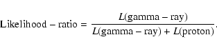$$% {\rm Likelihood-ratio}=\frac{L({\rm gamma-ray})}{L({\rm gamma-ray})+L({\rm proton})}.$$ (1)

We took care to take account of the energy dependences of these two image parameters. An example of the Width parameter is shown in Fig. 12.

	Figure 12: Correlation between the Width and the logarithm of total ADC counts obtained from the gamma-ray simulations.
Open with DEXTER

In order to correct for the energy dependence, we made 2D-histograms, i.e., the shape parameter versus the logarithm of the total ADC counts, and calculated PDFs for an energy independent acceptance of signal events. Here, we did not use either the Distance or Asymmetry parameter, as these parameters are source-point dependent. If the gamma-ray emitting region is broader than that of a point source, these parameters will deviate from that of point source. In the Monte-Carlo simulations for the PDF determination, we used the point-source assumption.

We selected gamma-ray-like events using the Likelihood-ratio. The Likelihood-ratio distributions are shown in Fig. 13.

	Figure 13: Likelihood distribution: a) for 2000 data and b) for 2001 data. "N'' denotes the number of events. The blank histograms are OFF-source data and the hatched areas are from the gamma-ray simulations.
Open with DEXTER

The signal peaks at a Likelihood-ratio of 1 and the background at 0.

We then investigated the figure of merit (FOM) using these data in order to maximize the statistical significance of the gamma-ray signals from NGC 253. At various cut locations, the signal of the Monte-Carlo simulation and the OFF background entry were obtained. The FOM was defined as the former value divided by the square root of the latter value. The FOM versus Likelihood-ratio cut values are plotted in Fig. 14. The figure suggests that higher cut values lead to a higher statistical significance, albeit with a loss in the gamma-ray acceptance. As a compromise between the acceptance and the FOM, we opted to adopt a value of 0.4 for the Likelihood-ratio cut, noting that there was only a small change in FOM between 0.2 and 0.6.

   
3.6 Further hot pixel rejection

Pixels occasionally have anomalously high trigger rates, often due to enhanced starlight or man-made light in the FOV of the pixel, or to small discharges between the light-guide and the photo cathode (Kabuki et al. 2002), or to electrical noise in the associated circuitry. Although these are generally random, small pulse-height signals, the high pixel trigger rates can have the affect of increasing the camera trigger rate. When randomly triggered during a real event trigger, these "hot pixels'' rarely form a cluster. Their effect was thought to be reduced after the pre-selection clustering cuts. However, it is possible that outlying hot pixels surviving the pre-selection cuts deform the shapes of the shower images. Such effects could significantly smear the $\alpha$ distribution for gamma-ray events. In fact, the $\alpha$ distributions of the OFF-source runs were observed to be deformed from the Monte-Carlo prediction.

	Figure 14: FOM (figure of merit) vs. Likelihood-ratio cut for the combined-data is shown by the solid line. Also shown is the acceptance vs. Likelihood-ratio cut (the dashed line).
Open with DEXTER

In order to flatten these distributions, we removed hot pixels. First we looked at the hot pixel map for events passing selection cuts. This enabled the hottest pixels to be identified and removed. We then looked at the scaler counts for the remaining pixels. In the same way, some of the hottest pixels were removed. Finally, we tested pixels iteratively to find out whether they deformed the $\alpha$ distributions of OFF-source run events for clusters having a center of gravity around the pixel being investigated. For the 2000 data, 12.3% of the pixels were removed by these operations. The same procedure was carried out for the 2001 data, and 9.7% of pixels were removed.

After removing those hot pixels, we checked theMonte-Carlo simulation precisely, and verified that these procedures did not result in any deformation of the image parameters, including $\alpha$.

Most of hot pixels were located around the edges of the camera. This occurred as PMTs with high trigger rates, which were identified early during camera testing, and were deliberately moved from inside the trigger region to the outer edge of the camera to minimize the effect on the hardware trigger.

In order to check whether small pulse-height random-noise signals were removed by these operations, we loosened the clustering to t3a, which should be more sensitive to these backgrounds. Similar plots were obtained, which confirmed that they were still consistent with the Monte-Carlo predictions. With t4a clustering and these procedures, we concluded that the random noises were removed successfully by this operation.

3.7 Results

The resulting $\alpha$ distributions are shown in Fig. 15.

	Figure 15: The distributions of $\alpha$ obtained for a) 2000 data and b) 2001 data. The points with error bars were obtained from ON-source data. The shaded histogram is from the OFF-source data.
Open with DEXTER

The excesses at $\alpha <$ 30$^\circ$ are 742.5 $\pm$ 104.6 events (7.1$\sigma$) for 2000 and 933.1 $\pm$ 106.2 events (8.8$\sigma$) for 2001, respectively. By combining the two years of data, the total excess was found to be 1651.9 $\pm$ 149.2 (11.1$\sigma$). Here, we used an Likelihood-ratio cut of 0.4. The $\alpha$ cut at 30$^\circ$ was larger than expected for a point source. This cut value was used in the previous detection of gamma-rays from RX J1713.7-3946, which was found to have an extended nature (Enomoto et al. 2002b). The distortion of the $\alpha$ spectrum in both ON- and OFF-source runs was observed in 2001 (Fig. 15b). The ON and OFF spectra, however, agreed well for $\alpha > 30^{\rm o}$, even including the normalization factor, which is described in Sect. 4.1. These appeared in higher $\alpha$ regions, and were considered to be due to hot channels which remained even after the rejection procedure described in the previous section. Most of these hot channels were located outside of the trigger region. In order to keep the high efficiency of the analysis, the hot channels which had less affect on the deformation of the $\alpha$ spectrum were not removed. For a point source, simulations predict that an $\alpha$ cut of between 15 and 20$^\circ$ should optimize the signal. The simulations indicate that 73% of the excess from a point source should have $\alpha < 15^{\circ}$. We tested $\alpha$ cuts from 15 to 35$^\circ$ in 5$^\circ$ steps in order to maximize the excess for this source, and found that 30$^\circ$ was best. The statistical significance of the signal thus needs these 5 trials to be taken into account. The final significance remained greater than 10$\sigma$. The signal rates were (743 $\pm$ 105) events/ 1301 min = 0.57 $\pm$ 0.08 for 2000 and (933 $\pm$ 106) event/ 1658 min = 0.56 $\pm$ 0.06 for 2001, consistent within the statistical errors. The average event rate overall was 0.56 $\pm$ 0.05 /min.

3.8 Various checks

We investigated the effect of raising the Likelihood-ratio cut, 0.6, i.e., applying a tighter cut. The results for the combined (2000 and 2001) data set are shown in Fig. 16b.

	Figure 16: $\alpha$ distributions obtained with a) the loose cut (L > 0.4), b) a tighter cut (L > 0.6), and c) "standard'' cuts. The points with error bars were obtained from ON-source data. The shaded histogram represents OFF-source data.
Open with DEXTER

The excess for the tight cut is 823.8 $\pm$ 105.6 (7.8$\sigma$), somewhat lower, as expected due the reduced acceptance.

In order to verify the Likelihood method, we checked the results of the "standard'' analysis, using an acceptance cuts of 0.05 < Width < 0.15 and 0.05 < Length < 0.3. The $\alpha$ distributions are shown in Fig. 16c. The excess is 1696.7 $\pm$ 165.9 (10.2$\sigma$), with signals of 811.7 $\pm$ 119.0 events (6.8$\sigma$) and 916.7 $\pm$ 115.4 events (8.0$\sigma$) in 2000 and 2001, respectively. As expected, the standard analysis confirms the statistical significance of the detection, though at a lower level than the more powerful Likelihood-ratio method.

3.9 Effective area

The effective areas for this analysis is shown in Fig. 17.

Figure 17: Effective area versus energy; a) effective areas after the pre-selection (the black squares), those after the distance cut (the black triangles), those after the Likelihood-ratio cut (the blank circles), and those with $\alpha < 15^{\rm o}$ (the blank squares). The effective area for the Whipple telescope is shown by the line (after the distance cut). b)The effective areas multiplied by E-2.5 are shown in order to indicatethe threshold of the CANGAROO telescope.

Open with DEXTER

We compared them with that of Whipple (Fig. 6 in Mohanty et al. 1998), which are the effective areas after clustering and Distance cut, i.e., before image parameter cut. Our effective area agreed with Whipple, even with the energy dependences. According to Fegan (1996), the threshold of Whipple telescope was the same as ours.

4 Discussion

   
4.1 Crab analysis

We observed the Crab nebula in November and December, 2000, in order to check our energy and flux determination. The Crab nebula has a power-law spectrum over a wide energy range (Aharonian et al. 2000; Tanimori et al. 1998b). The elevation angle ranged from 34$^\circ$ to 37$^\circ$. Approximately 10 hours of ON- and OFF-data were used for analysis. The energy threshold was estimated from simulations to be $\sim$2 TeV. The excessed number of events was 405 $\pm$ 59 (6.8$\sigma$), as shown in Fig. 18a.

Figure 18: Results of the Crab analysis. The differential flux obtained for the Crab nebula is shown in b), together with previous observations. The points with error bars were obtained by this experiment. The dotted line is the HEGRA result and the dashed line is the CANGAROO-I result. The insert a) is the $\alpha$ distribution. The points with error bars are obtained from ON-source data and the histogram is from OFF-source data. The lower plot c) is a significance map. The 65%-contour is drawn with the our estimated angular resolution (the arrows: $\pm 1 \sigma$).

Open with DEXTER

The differential flux, shown in Fig. 18b, is consistent with results from HEGRA (Aharonian et al. 2000) and CANGAROO-I (Tanimori et al. 1998a) observations. We conclude that our energy and flux estimations are correct. In addition, we derived a cosmic-ray spectrum from background events and compared it with the known cosmic-ray flux. From these checks, the systematic uncertainty for the absolute flux estimation was found to be within 10%.

The $\alpha$ plot for the Crab nebula, shown as an insert (Fig. 18a, is consistent with the point-source assumption. The OFF-$\alpha$ spectrum was again not flat. The average image positions were different from the zenith-angle observation, i.e., they were centerized because the shower max position was higher in altitude. The reflective index of air was smaller there, which resulted in a smaller Cherenkov angle. In addition, there is a bright star close to the Crab position. In order to avoid a high trigger rate, we displaced (0.25 degrees) the telescope's tracking center away from the center position of the Crab nebula. The average hit region in the camera was different from the observation of NGC 253. Thus, a different $\alpha$ deformation (due to the hot channels) occurred in this case. The 65% contour obtained from the significance map is shown in the lower plot Fig. 18c. The arrows are the estimated angular resolution ( $\pm 1 \sigma$ = $\pm 0.25 ^\circ$). Note that this is larger than that of the NGC 253 analysis (0.23$^\circ$), due to the zenith-angle dependence. The Crab was observed at zenith angles of around 56$^\circ$, whereas NGC 253 was observed at around 6$^\circ$. The center of the significance map corresponds to the Crab pulsar, confirming that our pointing and angular resolution are consistent with our Monte-Carlo simulations.

Miscellaneous checks were carried out, as described here. The agreements between the ON and OFF $\alpha$ distributions in a region greater than 30 degrees were compared with the observation times listed in Table 3. The result is $\frac{N_{{\rm on}}/N_{{\rm off}}}{T_{{\rm on}}/T_{{\rm off}}}=1.02$ . The signal rate for each individual observation was calculated, and the results are plotted in Fig. 19.

	Figure 19: Excesses versus observation times (after cloud cut) for all runs. The blank marks were obtained by an OFF-source run, and the filled marks by ON-source runs. The dashed line is the average flux.
Open with DEXTER

They are consistent with the average flux described above.

4.2 Systematic uncertainty in the energy determination

There were uncertainties in determining the energy scale from the total ADC counts. The ADC conversion factor was 92 ⁺¹³_-7, as previously described. The mirror reflectivity also had some uncertainty, in both its value (averaged over the whole mirror) and its time dependence. A measure of the latter could be made from month-by-month shower rates. Also, Mie scattering was not taken into account in our Monte-Carlo simulations. Considering all of these effects, we estimated the systematic uncertainty in the energy determination to be within 15% (bin to bin) and 20% (overall). These are also consistent with the Crab analysis results described previously.

4.3 Differential flux

The energy spectra of TeV gamma-ray sources generally have a power-law nature. Therefore, we used the ${\rm log_{10}} (Energy)$ scale in binning events to determine the spectrum for NGC 253, rather than energy, itself. The energy for each event was assigned as a function of the total ADC counts, where the relation between the energy and the total ADC counts was obtained from simulations. The excess (gamma-ray) events were observed between 0.5 and 3 TeV. We divided this ${\rm log_{10}} (Energy)$ range using equipartition. The number of binnings is 6. In Fig. 20, the derived spectra for both 2000 and 2001 are plotted, and are seen to be consistent with each other.

	Figure 20: Differential fluxes for the 2000 and 2001 data. The blank squares represent data from 2000, and the filled squares are from the 2001 data. The triangles are the upper limits. The dotted line is that of Crab nebula for a reference.
Open with DEXTER

The systematic uncertainties were estimated as follows. The background light sources, such as stars and artificial light may have a significant effect on the estimation of the differential flux determinations. These backgrounds affect each pixels pulse-height distribution. Small contributions (Poisson distributed) would be added to the signal in each pixel. In order to study the significance of this effect, we varied the ADC threshold from 300 (default), to 350 and 400 (corresponding to 3.3, 3.8, and 4.3 p.e., respectively). The differential flux was obtained for each case and plotted in Fig. 21.

	Figure 21: ADC threshold dependence of the differential fluxes.
Open with DEXTER

The total excesses of signals varied 1652 $\pm$ 149 events (300 count threshold), 1429 $\pm$ 154 events (350), and 1034 $\pm$ 160 events (400), respectively. The acceptances were (as expected) strongly dependent on the threshold value, but the differential fluxes were stable, as shown in Fig. 21.

As a further check that the excess events are due to gamma-rays, the following tests were also made. We re-calculated the Likelihood-ratios by first adding asymmetry, then removing length, and finally, removing width. This was done to check whether only one parameter had an unduly large effect on the final signal. The resulting fluxes are shown in Fig. 22.

	Figure 22: Differential fluxes based on various assumptions concerning the Likelihood-ratios.
Open with DEXTER

A deviation was observed when we added asymmetry to the Likelihood-ratio. Asymmetry could only be calculated under the assumption of a point source at the center of the FOV. As we had already concluded that the source was extended, the fact that the use of asymmetry reduces the significance of the signal is not unexpected, and confirms that it is not a useful parameter for diffuse radiation. The other Likelihood-ratios were in agreement with each other, supporting our conclusion that the excess is due to diffuse gamma-ray emission. A summary of flux changes in this parameter study is listed in Table 4.

Table 4: Summary of the flux changes in the parameter study at each energy binnings.

The mean energies listed in this table were obtained by averaging the generated energies of the accepted events in the ADC binnings in the above-described Monte-Carlo simulation.

In order to derive the spectrum of NGC 253 self-consistently, we adopted the following method. The above spectrum was derived by using acceptances derived from simulations in which a E^-2.5 spectrum was assumed. If we fit the fluxes with a differential power-law spectrum, we obtained an index of -3.7 $\pm$ 0.3. We then iteratively used this value in simulations to re-derive the spectrum. This process rapidly converged at an index of -3.75 $\pm$ 0.27. The differential fluxes estimated with E^-2.5 input and that with E^-3.75 are shown in Fig. 23.

	Figure 23: Differential flux estimated by the various energy spectra inputs in the Monte-Carlo simulation. The blank squares were obtained by E-2.5, the black squares by E-3.75, and the black circles by the exponential cutoff function described in the text.
Open with DEXTER

Both showed the same best fit spectrum.

Table 5: Systematic errors and energy resolutions of each energy binning.

An extrapolation of this power-law spectrum to lower energies deviates greatly from the measured fluxes and upper limits (Blom et al. 1999; Sreekumar et al. 1994); a turn-over below the TeV region clearly exists. Physically plausible functions exist with a turn-over include spectra $\propto E^{-\gamma}e^{-E/E_{{\rm max}}}$ and $\propto E^{-\gamma}e^{-\sqrt{E}/a}$. Although the former is typically used for the spectra of gamma-rays originating from $\pi^{\rm o}$ decay, the value of $\gamma$ should be greater than 2.0 according to the present acceleration theories, in contradiction with the measurements at lower energies. The latter form is typical for an Inverse Compton origin. We fitted a spectrum of this form with the EGRET upper limits. The best fit with this function gave a=0.28 with a reasonable $\chi^2$ value. We tried to generate events with this spectral input to derive the differential flux again. These are shown in Fig. 23 (the black circles). The flux determination is very stable over a range of assumptions for the Monte-Carlo inputs of the energy spectrum. We also carried out an iteration with this function, and confirmed the convergence to be good. Finally, we selected this to be the Monte-Carlo energy spectrum.

The systematic errors were estimated by varying the Likelihood-ratio cut values, as described previously. They are listed in Table 5. These values are larger than those in Table 4. We, therefore, concluded to use these as the systematic errors. Also shown are the energy resolutions in each bin, which were obtained from simulations on an event-by-event basis. These errors are dominated by the core distance uncertainties. From here on, the flux errors in the figures are the square root of the quadratic sum of the statistical and systematic errors.

The combined flux is shown in Fig. 24 and Table 6.

	Figure 24: Combined differential fluxes. The dotted line is that of Crab nebula observations. The other lines are the fitting results. The dashed line is that of a power-law. The solid curve is that with an exponential cutoff.
Open with DEXTER

Around 1 TeV, the flux is about one order lower than in the Crab nebula, which is indicated by the dotted line in Fig. 20 (Tanimori et al. 1998a).

Table 6: Energy binnings and differential fluxes. The first errors are statistical and the second ones are systematic.

The goodness of fit for the various spectra were characterized by the $\chi^2$ values. The results for various fittings are as follows:

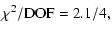$$\begin{eqnarray*}\frac{{\rm d}F}{{\rm d}E}&=&(2.85\pm 0.71)\times 10^{-12} \\ &... ...\rm 1~ TeV})^{(-3.85\pm 0.46)} ~{\rm [cm^{-2}~s^{-1}~TeV^{-1}]}, \end{eqnarray*}$$

$$% \chi^{2}/{\rm DOF}=2.1/4,$$ (2)

$$\begin{eqnarray*}\frac{{\rm d}F}{{\rm d}E}=a e^{\sqrt{E_0}/b} (E/E_0)^{-1.5}e^{-\sqrt{E}/b} ~{\rm [cm^{-2}~s^{-1}~TeV^{-1}]}, \end{eqnarray*}$$

$$\begin{eqnarray*}a=6 \times 10^{-5}~{\rm [cm^{-2}~s^{-1}~TeV^{-1}]},~E_0=0.0002~{\rm TeV}, \end{eqnarray*}$$

 

$$% b=0.25 \pm 0.01~[\sqrt{\rm TeV}], \chi^{2}/{\rm DOF}=1.8/5,$$ (3)

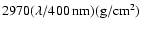
where the second formula is based on the Inverse Compton scattering formula when we constrain the flux at 3/4 of the EGRET upper limit at E₀= 0.0002 TeV. Due to this, the two parameters in Eq. (3), a and E₀, were fixed to those values. Here we assumed the power law index of the incident electron energy spectrum to be 2.0. A better $\chi^2$ was obtained for this fit compared to the single power-law fit. In order to explain our flux and that of EGRET simultaneously, Eq. (3) is one of reasonable choices.

4.4 Morphology

The thick contours in Fig. 25 represent the source morphology obtained from our observations.

	Figure 25: Significance map obtained by this experiment, shown by the thick contours. The thin contours are optical image by DSS2.
Open with DEXTER

These contours were obtained from the so-called significance map and are, therefore, not exactly speaking a morphology. The significance map was made from the distribution of the detection significance determined at each point, based on the assumption that each point in turn was a point-source position. The significance was obtained from the difference in the $\alpha$ plot (ON- minus OFF-source histogram) divided by the statistical errors. The angular resolution of this method was estimated to be $0.23^{\circ}$ (1$\sigma$ is a 68% confidence level). The telescope pointed at the center of NGC 253. Also shown by the thin contours is an optical image obtained by DSS2 (second version of Digital Sky Survey). The "Significance'' is proportional to the intensity only when the acceptance and the background level are uniform in the full FOV. The detection efficiency is dependent on the offset angle of the assumed source position from the centre of the field of view, as shown in Fig. 26.

	Figure 26: Efficiency versus offset angle of the gamma-ray source position from the center of the field of view.
Open with DEXTER

We checked the effect of the background light. The optical magnitude of NGC 253 has magnitudes of $m_{\rm B} \sim 8$ and $m_{{\rm vis}} \sim 7.1$. Even if it was concentrated on one point, the background level due to this was lower than our sensitivity (Stars fainter than a magnitude of 5 could not be detected in either the scaler or ADC data). We also note that the lower cut on Distance was 0.5$^\circ$, and so pixels around the center of NGC 253 were generally not used for the analysis. When observing NGC 253, the brightest stars in the FOV have magnitudes of 5.6. However, we observed some effects from a group of faint stars (each of magnitude $\sim$6) in observations of another target, which deformed the shapes of the parameter distributions. These effects are believed to be removed by the hot pixel rejection algorithm, described in Sect. 3.6. This was demonstrated in an analysis of the Crab nebula data. Although the visual magnitude of the Crab nebula is 8.4, a bright star (magnitude 3.1) is located within the FOV of our camera. Despite this, we were able to derive a significance map consistent with the other measurements (Fig. 18). Because we cannot rule out the possibility that "hot pixels'' may deform the significance map, we can not definitely derive the morphology of the gamma-ray emitting regions from observations with only a single telescope.

Figure 27 shows the acceptance of gamma-ray-like events as a function of the Distance upper cut values (minimum cut is $0.5^{\circ}$).

	Figure 27: Signal yield as a function of the upper range of the Distance cut. The yield was normalized to the total excess. The points with error bars were obtained by this experiment. The solid line was obtained from a Monte-Carlo simulation with a point source assumption. The dashed line is the case for a "diffusion angle'' of 0.4$^\circ$.
Open with DEXTER

From this figure, we tried to estimate the spatial extent of the gamma-ray emission. We proceeded by fixing the minimum cut value of Distance at $0.5^{\circ}$ (as used in previous Whipple and CANGAROO analyses). The maximum cut value was varied between 0.6 and 1.5, and the excess events for each cut were plotted by the points with error bars.

We checked the consistency between the experimental data and the source diffusion assumptions. At first, the solid line in Fig. 27 was obtained by a Monte-Carlo simulation with a point-source assumption. The observed distribution is clearly broader than this.

From the significance map (Fig. 25), the correlations between the orientations of the TeV emission and optical image were calculated and the standard deviation of the long axis was 0.37$^\circ$ and of the short axis was 0.24$^\circ$, respectively. The long axis was inclined by +30$^\circ$ from the horizontal axis. This is slightly larger than that of the optical image; however, we do not believe that the difference is significant. An analysis of the map of the number excess events yielded similar results. We then carried out a Monte-Carlo simulation based on various assumptions. We varied the extent of the emitting region by smearing the gamma-rays' incident angle with a Gaussian. Our data are consistent with "diffusion angles" of between 0.3-0.6$^\circ$. The case of 0.4$^\circ$, shown in Fig. 27 by the dashed line, is consistent with the observation. However, it is necessary to wait for future stereo observations (CANGAROO-III and H.E.S.S.) before any quantitative estimates of the extent of the emission region can be made and the morphology studied. We can concluded that the emission is consistent with Gaussians between 0.3-0.6$^\circ$, which correspond to 13-26 kpc at a distance of 2.5 Mpc. Changing the input gamma-ray's spatial distribution from Gaussian to a rectangular shape gave similar results, i.e., Fig. 27 can be reproduced by a 0.4$^\circ$ rectangular spatial emission. This can be understood by the efficiency reduction due to the limited FOV. The acceptance for our telescope was reduced from an offset angle of 0.5$^\circ$. The electrons of GeV energy associated with NGC 253 was reported by radio observations of Hummel et al. (1984) and Carilli et al. (1992). The size of the emission region is similar to our result. An interpretation of this results can be found in Itoh et al. (2003).

5 Conclusions

In this paper we have concentrated on technical details concerning our observations and analysis. Statistically significant signals of gamma-rays from the nearby starburst galaxy NGC 253 have been detected. The differential flux shows a turnover below 0.5 TeV. The spatial distribution of the gamma-ray emission is broader than that of a point-source. This is consistent with a width of 0.3-0.6$^\circ$, corresponding to 13-26 kpc at the location of NGC 253. A more detailed physical interpretation is presented elsewhere (Itoh et al. 2003).

Acknowledgements

We thank Prof. T. G. Tsuru for help to analyze the multi-wavelength observational results. This work was supported by a Grant-in-Aid for Scientific Research by the Japan Ministry for Education, Science, Sports, and Culture, Australian Research Council, and Sasagawa Scientific Research Grant from the Japan Science Society. The support of JSPS Research Fellowships for A.A., J.K., K.O. and K.T. are gratefully acknowledged. The Digitized Sky Survey was produced at the Space Telescope Science Institute under U.S. Government grant NAG W-2166. The images of these surveys are based on photographic data obtained using the Oschin Schmidt Telescope on Palomar Mountain and the UK Schmidt Telescope. The plates were processed into the present compressed digital form with the permission of these institutions.

References

 
• Aharonian, F. A., Akhperjanian, A. G., Barrio, J. A., et al. 2000, ApJ, 539, 317 In the text NASA ADS  
• Antonucci, R. R. J., & Ulvestad, J. S. 1988, ApJ, 330, L97 In the text NASA ADS  
• Baum, W. A., & Dunkelman, L. 1955, J. Opt. Soc. Am., 45, 166 In the text  
• Bhattacharya, D., The, L.-S., Kurfess, J. D., et al. 1994, ApJ, 437, 173 In the text NASA ADS  
• Blom, J. J., Paglione, T. A. D, & Carraminana, A. 1999, ApJ, 516, 744 In the text NASA ADS  
• van Buren, D., & Greenhouse, M. A. 1994, ApJ, 431, 640 In the text NASA ADS  
• Carilli, C. L., Holdaway, M. A., Ho, P. T. P., & de Pree, C. G. 1992, ApJ, 399, L59 In the text NASA ADS  
• Enomoto, R., Tanimori, T., Asahara, A., et al. 2001, Proc. 27th ICRC (Hamburg) 6, 2477 In the text  
• Enomoto, R., Hara, S., Asahara, A., et al. 2002a, Astropart. Phys., 16, 235 In the text NASA ADS  
• Enomoto, R., Tanimori, T., Naito, T., et al. 2002b, Nature, 416, 823 In the text NASA ADS  
• Fegan, D. J. 1996, Space Sci. Rev., 75, 137 In the text NASA ADS  
• Goldshmidt, O., & Rephaeli, Y. 1995, ApJ, 444, 113 In the text NASA ADS  
• GEANT, CERN Program Library Long Write up W5013 In the text  
• Hillas, A. M. 1985, Proc. 19th. ICRC (La Jolla), 3, 445 In the text  
• Hara, T., Kifune, T., Matsubara, Y., et al. 1993, Nucl. Instr. Meth. A, 332, 300 In the text  
• Hara, S. 2002, Ph.D. Thesis, Tokyo. Inst. Tech., unpublished In the text  
• Hummel, E., Smith, P., & van der Hulst, J. M. 1984, A&A, 137, 138 In the text NASA ADS  
• Itoh, C., Enomoto, R., Yanagita, S., Yoshida, T., et al. 2002, A&A, 396, L1 In the text NASA ADS  
• Itoh, C., Enomoto, R., Yanagita, S., Yoshida, T., & Tsuru, G. 2003, ApJ, 584, L65 In the text NASA ADS  
• Jelley, J. V. 1958, Cerenkov Radiation and its Applications (New York: Pergamon Press), 219 In the text  
• Kabuki, S., Tsuchiya, K., Okumura, K., et al. 2002, Nucl. Instr. Meth. A., to appear [asrto-ph/0210254] In the text  
• Kawachi, A., Hayami, Y., Jimbo, J., et al. 2001, Astropart. Phys., 14, 261 In the text NASA ADS  
• Kifune, T., Tanimori, T., Ogio, S., et al. 1995, ApJ, 438, L91 In the text NASA ADS  
• Kubo, H., Asahara, A., Bicknell, G. V., et al. 2001, Proc. 27th ICRC (Hamburg), 5, 2900 In the text  
• Mattila, S., & Meikle, W. P. S. 2001, MNRAS, 324, 325; Erratum 327, 350 In the text NASA ADS  
• Mohanty, G., Biller, S., Carter-Lewis, D. A., et al. 1998, Astropart. Phys., 9, 15 In the text NASA ADS  
• Muraishi, H., Tanimori, T., Yanagita, S., et al. 2000, A&A, 354, L57 In the text NASA ADS  
• Okumura, K., Asahara, A., Bicknell, G. V., et al. 2002, ApJ, 579, L9-12 In the text NASA ADS  
• Sreekumar, P., Bertsch, D. L., Dingus, B. L., et al. 1992, ApJ, 400, L67 In the text NASA ADS  
• Sreekumar, P., Bertsch, D. L., Dingus, B. L., et al. 1994, ApJ, 426, 195 In the text  
• Tanimori, T., Sakurazawa, K., Dazeley, S. A., et al. 1998a, ApJ, 492, L33 In the text NASA ADS  
• Tanimori, T., Hayami, Y., Kamei, S., et al. 1998b, ApJ, 497, L25 In the text NASA ADS  
• de Vaucouleurs, G. 1978, ApJ, 224, 710 In the text NASA ADS  
• Voelk, H. J., Klein, U., & Wielebinski, R. 1989, A&A, 213, L12 In the text NASA ADS  
• Voelk, H. J., Aharonian, F. A., & Breitschwerdt, D. 1996, Space Sci. Rev., 75, 279 In the text NASA ADS