A&A 402, 541-547 (2003)
DOI: 10.1051/0004-6361:20030166
Photometric parallaxes of Southern high proper motion stars. I.
E. Costa1 - R. A. Méndez2
1 - Departamento de Astronomía, Universidad de Chile, Casilla 36-D,
Santiago, Chile
2 - European Southern Observatory, Casilla 19001, Santiago 19, Chile
Received 25 October 2002 / Accepted 7 January 2003
Abstract
Photometric distances derived from VRI photometry are given
for 44 high proper motion stars from the Cerro El Roble proper motion
surveys of Wroblewski & Torres and Wroblewski & Costa. The
observations were carried out with the main purpose of estimating the
distance of selected members of the above survey that are likely to be
nearby. We have discovered 13 stars closer than 25 pc, the classical
limit of the Catalogs of Nearby Stars (see e.g. Gliese &
Jahrei 1991) and the NASA/NSF NStars Project. Those stars of
the sample whose photometric distances are less than
1991) and the NASA/NSF NStars Project. Those stars of
the sample whose photometric distances are less than  25 pc, or
have proper motions in excess of 0.50 arcsec/year, are either
currently being targeted by the Cerro Tololo Parallax Investigation
(CTIOPI) or will be targets of a forthcoming expansion of this survey.
25 pc, or
have proper motions in excess of 0.50 arcsec/year, are either
currently being targeted by the Cerro Tololo Parallax Investigation
(CTIOPI) or will be targets of a forthcoming expansion of this survey.
Key words: astrometry - stars: kinematics - techniques: photometric
The nearest stars, being the brightest examples of their types, provide
astronomers with much of our understanding of stellar astronomy. For
most types of stars, the fundamental framework of stellar astronomy is
built upon direct measurements of luminosities, colors, temperatures,
and masses of nearby stars.
The faint members of the solar neighborhood are however significantly
underrepresented. Using the Research Consortium on Nearby Stars updated
list of stars closer than 10 pc (see Henry 2003), and assuming
that the density of stellar systems within 5 pc (44 systems) carries to 10 pc,
it can be estimated that 125 (36%) systems are missing from the current 10
pc census. The problem is obviously worse to 25 pc, a distance at which the
incompleteness can be predicted to be as much as 60%.
Unfortunately there is no simple way to deal with this situation; only large
trigonometric parallax programs could remedy the problem. Furthermore, for such
surveys to be efficient, their input target lists must be as refined as possible,
so candidate nearby stars must be carefully selected on the basis of some
"closeness'' indicator; such as having a high proper motion and/or a
photometric estimate of their distance.
With the above immediate purpose in mind, and within the scope of the
Cerro Tololo Parallax Investigation (CTIOPI, Henry et al. 1999), a
southern hemisphere trigonometric parallax survey whose goal is to
increase the population of stars known within 25 pc of the Sun by
20%, along with a forthcoming expansion of the CTIOPI effort, we
started a program to determine photometric distances of high proper
motion stars from the Cerro El Roble (EACR) proper motion surveys of
Wroblewski & Torres (hereafter W&T, see e.g. A&AS 122, 447, 1997)
and Wroblewski & Costa (hereafter W&C, see e.g. A&A 367, 725,
2001).
In the course of the EACR surveys, 2495 new stars with proper motions
larger than 0.15 arcsec/year were discovered and 1262 Luyten
Catalogue (LTT, Luyten 1957) were re-discovered, so, for our program
to be realistic, it was necessary to pre-select the candidates for the
photometry. This was done essentially on the basis of their proper
motion, the faster being more important. Because of their possible
astrophysical importance, the highest ranked objects were those that
are both fast moving and faint. After excluding objects with
known parallaxes (mainly bright stars), and those being targeted by
the photometric survey of Ianna et al. (see e.g. Patterson et al. 1998), a priority ranking including some 200 stars was created.
It should be noted that roughly 10% of the stars in our working list
are currently being observed by CTIOPI, and a similar additional
percentage will be targeted by the forthcoming extension of this
survey.
In this first paper we give photometric distances, based on VRI photometric
observations made with the 0.9 m telescope Cerro Tololo Interamerican Observatory
(CTIO), for part of the brighter sample of WT/LTT stars in our list. Coordinates
and finding charts for the 44 objects observed can be found - as indicated in Table 1 -
in the series of papers of the EACR survey (it should be noted that the LTT
catalogue does not include finders). In a second contribution being prepared,
we will present results for the fainter sample, based mainly on observations
carried out with the CTIO 1.5 m telescope.
The observations were made with a Tektronic
 CCD detector with
24
CCD detector with
24 pixels attached to the Cassegarin focus of the CTIO 0.9 m telescope.
This combination gives a field size of 1
pixels attached to the Cassegarin focus of the CTIO 0.9 m telescope.
This combination gives a field size of 1
 and a scale of 0.396
 /pixel. The inverse gain was 1.5 e-/ADU,
and the corresponding read noise 3.6 e-.
/pixel. The inverse gain was 1.5 e-/ADU,
and the corresponding read noise 3.6 e-.
Our VRI instrumental photometric system was defined by the use of the
following filters: Vtek2: 5475/1000, Rtek2: 6425/1500 and I-KC#31:
8075/1500 (where the first figure is the measured central wavelength
of the filter and the second its FWHM, in A). These filters
constitute the default option on the 0.9 m telescope for broad-band
photometry on the standard VRI Johnson-Kron-Cousins system.
Additional information about them, including their transmission
curves, can be found in http://www.ctio.noao.edu/instruments/filters/index.html
Typically 6 UBVRI standard star areas from the catalogs of Landolt
(1992) and Graham (1982) were observed multiple times each night to
determine the transformation of our instrumental magnitudes to the
standard VRI system. Although most of these areas include stars of a
wide variety of colors, given the presumably very red colors of most
of our targets, very red standards were observed additionally. A few
of the standard areas were followed each night up to about 2.2
airmasses to optimally determine atmospheric extinction.
All program stars were observed during transit, following the sequence
VRIIRV. Although time consuming, this latter practice has proved very
useful to check for consistency.
All CCD frames were first calibrated using standard IRAF (version
2.11.3, NOAO, University of Arizona) tasks. For this purpose Zero
exposures and Twilight Sky Flats were taken every night.
Aperture photometry was then performed on each object of interest
using the IRAF APPHOT package. The optimum aperture size for each
night, ensuring a negligible loss of light from the PSF wings and
minimizing light contamination from close objects, was determined by
means of the IRAF MKAPFILE task. The best aperture radius turned out
to be 4-5 times the average FWHM of the frames.
To put our observations into the standard system, we used the
following transformation equations:
where (v, r, i) and (V, R, I) are the instrumental and standard magnitudes
respectively, (Xv, Xr, Xi) are the airmasses and v1, v2,
v3, v4, etc. are constants. It should be noted that in the
absence of blue-passband observations it was not possible to use (as
is the common practice) the (B-V) color for the standardization of the
v magnitude. As shown previously by Bucciarelli et al. (2001), the
(B-V) and (V-R) colors of the Landolt stars are linearly related and
comparable in range, so the use of the (V-R) color in the (v,V)
equation is equally satisfactory.
Equations (1) were applied to the Landolt/Graham standard star
magnitudes, and solved using the IRAF FITPARAMS task, which performs a
least-square fit to the system. This task can be run interactively,
which permits the rejection of problematic observations to control the
quality of the fit. Without major massaging, the rms of all fits
turned out to be around 0.02 mag. With the exception of the
second-order color terms coefficients (v4, r4, i4) the formal
errors of the calculated coefficients were significantly smaller than
their derived values.
Finally, the above set of transformation equations - with their
corresponding calculated coefficients - was applied to our program
stars for their calibration. This was done by means of the IRAF
INVERTFIT task, which produces a set of calibrated magnitudes and
colors and their errors: in the present case specifically: V,
error (V), (V-R), error (V-R) and (V-I), error (V-I). As pointed out by
Bucciarelli et al. (2001), the final photometric error computed by
INVERTFIT does not rigorously treat error propagation, therefore
producing a lower limit of the photometric errors.
The results of our VRI photometry are presented in Table 1. The first
column gives the name of the star in the EACR survey (the "WT'' number)
or its name in the LTT Catalogue; the second column the number of
times the star was observed; Cols. 3, 6 and 9 their average Vmagnitude and (V-R) and (V-I) colors, respectively; Cols. 4, 7 and 10 the square root of the sum of the squares of the IRAF-computed
errors of each observation for V, (V-R) and (V-I), respectively;
Cols. 5, 8 and 11 the standard deviation of the average values of V,
(V-R) and (V-I), respectively. These errors have to be interpreted
with caution; it must be kept in mind that they have been derived from
a small number of independent measures. They have been included here
for comparison with the lower limit error given by IRAF, and because
they are the starting point to determine the propagation of errors
described in Sect. 6. It should also be noted that high photometric
errors in (V-R) and (V-I) usually just reflect a poor
determination of the V magnitude; this is because - these stars being
in general quite brighter in the R and I bandpasses - their R, Imagnitudes are precisely determined. Finally, Col. 12 gives the
reference to the W&T or W&C paper where coordinates, proper motion,
position angle, and a finding chart can be found for the star. An
asterisk in the Remarks column indicates that additional comments are
made in Sect. 5 (Notes on individual objects).
Table 1:
VRI Photometry of Southern high proper motion stars from the Cerro El
Roble proper motion survey.
WT233: two objects are now seen near the position indicated for
this star by the W&T finding chart (see W&T, A&AS 91, 129, 1991).
The W&T finder was made from a Maksutov Astrograph plate (scale:
 /mm) taken circa 1990, and shows only one object; because
at that epoch one star was eclipsing the other. On account of the
proper motion that occurred in the roughly 10 year epoch difference
between that plate and our photometry (plus the better scale of the
photometry frames), two objects are now clearly distinguished. We
identify the brightest and reddest of them, "WT233b'' in Tables 1 and 2, as the correct W&T star. The fainter object,"WT233f" in those
tables, lies 9
to the SE. This object is bluer and
seems to be variable. It is interesting to note that the variability
is most notable in the I and R bandpasses. In Fig. 1 we give a
finding chart produced from a photometry frame.
/mm) taken circa 1990, and shows only one object; because
at that epoch one star was eclipsing the other. On account of the
proper motion that occurred in the roughly 10 year epoch difference
between that plate and our photometry (plus the better scale of the
photometry frames), two objects are now clearly distinguished. We
identify the brightest and reddest of them, "WT233b'' in Tables 1 and 2, as the correct W&T star. The fainter object,"WT233f" in those
tables, lies 9
to the SE. This object is bluer and
seems to be variable. It is interesting to note that the variability
is most notable in the I and R bandpasses. In Fig. 1 we give a
finding chart produced from a photometry frame.
WT1289: there is a very faint red object 7
to the
SE of this star, which is not visible in the W&T finder. Photometry was not
possible due to its faintness.
WT1760: two objects are now seen near the position indicated for
this star by the W&T finding chart (see W&T, A&AS 122, 447, 1997).
The W&T finder was made from an image extracted from the Digitized
Sky Survey (produced by the Space Telescope Science Institute), which
was in turn obtained from a UK Schmidt Telescope plate (scale:
 /mm) taken circa 1980, and shows one object because at
that epoch one star was eclipsing the other. On account of the proper
motion that occurred in the roughly 20-year epoch difference between
that plate and our photometry (plus the better scale of the photometry
frames), two objects are now clearly distinguished. We identify the
brighter and much redder object, "WT1760b'' in Tables 1 and 2, as the
correct W&T star. The bluer and fainter object (not included in
those tables), lies 11
to the NW. For this latter,
which seems to be variable, we obtained moderate precision photometry:
V=16.94, error (V)=0.04;
(V-R)=0.42, error
(V-R)=0.06;
(V-I)=0.81,
error
(V-I)=0.09 (IRAF-computed errors). In Fig. 2 we give a finding
chart produced from a photometry frame.
/mm) taken circa 1980, and shows one object because at
that epoch one star was eclipsing the other. On account of the proper
motion that occurred in the roughly 20-year epoch difference between
that plate and our photometry (plus the better scale of the photometry
frames), two objects are now clearly distinguished. We identify the
brighter and much redder object, "WT1760b'' in Tables 1 and 2, as the
correct W&T star. The bluer and fainter object (not included in
those tables), lies 11
to the NW. For this latter,
which seems to be variable, we obtained moderate precision photometry:
V=16.94, error (V)=0.04;
(V-R)=0.42, error
(V-R)=0.06;
(V-I)=0.81,
error
(V-I)=0.09 (IRAF-computed errors). In Fig. 2 we give a finding
chart produced from a photometry frame.
LTT1588: there is a moderately faint red object, clearly
visible in the W&C finder, 10
to the NE of this star. We could
only secure low-precision photometry of it: V=16.63, error (V)=0.11;
(V-R)=0.97,
error
(V-R)=0.12;
(V-I)=1.96, error
(V-I)=0.12 (IRAF-computed errors).
![\begin{figure}
\par\resizebox{\hsize}{!}{\includegraphics[clip]{3233.f1.eps}} \end{figure}](/articles/aa/full/2003/17/aa3233/Timg16.gif) |
Figure 1:
Finding chart for WT233. Chart is 4.1 arcmin on a
side; North is at the top, East to the left. The object marked with
ticks, which we identify as the W&T star, is WT233b in Tables 1 and
2. The fainter object immediately to the SE is WT233f. See Sect. 5
for details. |
| Open with DEXTER |
![\begin{figure}
\par\resizebox{\hsize}{!}{\includegraphics[clip]{3233.f2.eps}} \end{figure}](/articles/aa/full/2003/17/aa3233/Timg17.gif) |
Figure 2:
Finding chart for WT1760. Chart is 4.1 arcmin on a
side; North is at the top, East to the left. The object marked with
ticks, which we identify with the W&T star, is WT1760b in Tables 1
and 2. The fainter object immediately to the NW is that alluded to in
Sect. 5. |
| Open with DEXTER |
In this section we discuss the methods employed to obtain photometric
parallaxes, using the VRI photometry described in the previous sections.
Photometric distances have been determined in two semi-independent
ways: using a relationship between MV and (V-R) on one hand, and
between MV and (V-I) on the other. These relationships have been
derived by T. Henry (private communication), using the latest data
available in the Research Consortium on Nearby Stars (RECONS)
database, which contains trigonometric parallaxes and good photometric
data for about 140 stars closer than 10 pc (see
http://www. chara.gsu.edu/~thenry/RECONS). The above
relationships are valid in the spectral type range from about G5 to
M8, which corresponds to a range of 0.37-2.20 in (V-R), a range of
0.55-4.70 in (V-I), and an absolute magnitude range of
 .
As shown by Table 1, some stars in our sample have colors
slightly bluer than those allowed by the relationships derived by
Henry; in these few cases we used fits derived from the tabulations
provided by Schmidt-Kaler (1986, Table 13) and Schneider (1996,
Table 9) to obtain MV.
.
As shown by Table 1, some stars in our sample have colors
slightly bluer than those allowed by the relationships derived by
Henry; in these few cases we used fits derived from the tabulations
provided by Schmidt-Kaler (1986, Table 13) and Schneider (1996,
Table 9) to obtain MV.
![\begin{figure}
\par\includegraphics[width=15.5cm,clip]{3233.f3.eps} \end{figure}](/articles/aa/full/2003/17/aa3233/Timg19.gif) |
Figure 3:
Color-color diagram for our stars compared to various
fiducial lines. Note the unequal size of both axis, which makes it
appear as if the errors in (V-R) are larger than those in (V-I),
whereas in fact they are comparable. The solid line comes from Table
9 in Schneider (1996), which gives colors computed from Vilnius
spectra. The dashed line is from Bessell (1995), and it is based on a
combination of model and empirical model atmospheres for mid-K to late
M-type stars. The dot-dashed line is from the Palomar/MSU
spectroscopic survey of nearby stars by Hawley's et al. (1996), while
the dotted line is from an empirical calibration presented by Drilling
& Landolt (2000, Table 15.3.3). As it can be seen, the agreement
between all these fiducial lines and our data is quite good, and
within our observational errors. The four blueish stars marked in the
plot are discussed further in the text. |
| Open with DEXTER |
Given the faintness and large proper motion of the stars of our
sample, it is very unlikely that there are giants or sub-giants among
them; but, since all of the above relationships are valid only
for main-sequence stars, before deriving the photometric distances of
our targets we verified that they indeed appear to satisfy the above
relationships. This was accomplished by plotting our targets on a
color-color diagram, and superimposing fiducial lines for main
sequence stars, the result of which is presented in Fig. 2. As can
be seen from this figure, all our stars follow the expected main
sequence locus, and thus, it is justified to apply the relationships
mentioned above to derive their absolute magnitudes.
Since we have data with various degrees of accuracy in its photometry
(see Table 1), we have used a Monte-Carlo approach to derive the
photometric distances. Each star has a mean color and an associated
error for this color. These two values are used in a simulation to
derive many plausible photometric distances. After an appropriate
number of simulations has been done (defined as the number of
simulations for which both the mean distance and the distance
dispersion does not change significantly as we run more simulations,
see below), a mean value and a scatter for the distance is computed.
The final scatter in the derived distances is thus related to the
accuracy in the input photometric data exclusively.
In this method we assume that the absolute magnitude vs. color
relationship has a scatter smaller than that introduced by the
accuracy of our photometry. While this might be true for stars of a
given (fixed) metallicity, the natural spread in metallicity for Disk
stars adds an extra scatter, which can account for up to 0.2-0.3 mag
in MI for a given (V-I) (Leggett 1992; Kirkpatrick et al. 1994). This "cosmic'' scatter, can therefore add a extra 14%
error to the derived photometric distances. This is further confirmed
by Henry (2003), who made a comparison of photometric and
trigonometric distances for 97 stars within 10 pc, which indicates
that the distance estimation technique utilized here results in
distances accurate to about 15%. However, since we have no
metallicity indicator, we do not have a way to account for this
effect.
The Monte-Carlo simulations mentioned above follow the same methods
outlined in Méndez & Ruiz (2000), although used in a quite
different context. Details of the simulations can be found in that
publication. Briefly, these simulations are important because of the
obvious non-linear relationship between photometric errors and
(photometric) distance errors. For each pair (COL,
 ), we generate many random colors following a Gaussian
distribution of width
centered around COL. For
each of these, a photometric distance is calculated. After many
distances have been generated in this way, a mean distance and an rms
distance is calculated, and this is repeated for every star. More
specifically, and following Méndez & Ruiz (2000), the value
adopted for the color is given by:
), we generate many random colors following a Gaussian
distribution of width
centered around COL. For
each of these, a photometric distance is calculated. After many
distances have been generated in this way, a mean distance and an rms
distance is calculated, and this is repeated for every star. More
specifically, and following Méndez & Ruiz (2000), the value
adopted for the color is given by:
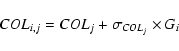 |
(2) |
where COLj is the (mean) observed color for star "j'' in the sample,
with measurement error
 ;
Gi the Gaussian
deviate (of zero mean and unity variance) for simulation "i'', and
COLi,j is the ith simulation value for the color of star j. The
no-errors situation is, of course, reproduced when all the Gi are
set to zero. The numbers of simulations is chosen such that the
variation in the derived mean distance and dispersion is quite small
(e.g., less than 1%), and it is typically less than 100 simulations
per star. Table 2 shows our results for the photometric distances and
the estimated dispersion as derived from each color; the weighted mean
is given in the last two columns.
;
Gi the Gaussian
deviate (of zero mean and unity variance) for simulation "i'', and
COLi,j is the ith simulation value for the color of star j. The
no-errors situation is, of course, reproduced when all the Gi are
set to zero. The numbers of simulations is chosen such that the
variation in the derived mean distance and dispersion is quite small
(e.g., less than 1%), and it is typically less than 100 simulations
per star. Table 2 shows our results for the photometric distances and
the estimated dispersion as derived from each color; the weighted mean
is given in the last two columns.
Table 2:
Photometric distances and its dispersion (all in pc) as
derived from data in Table 1.
Inspection of Table 2 shows that, in general, there is a very good
agreement between the distances derived from each color separately; in
most cases the differences are within  of the estimated
distance dispersion. We must note however that the two methods for
estimating the distances are not completely independent. The (V-R)and (V-I) colors rely on identical V magnitudes, so these colors are
semi-independent. While one could argue that the MV values (that
are responsible for most of the scatter through its intrinsic
metallicity scatter) depend on the same parallax measurement for both
relations, it is also evident that one has fitted
of the estimated
distance dispersion. We must note however that the two methods for
estimating the distances are not completely independent. The (V-R)and (V-I) colors rely on identical V magnitudes, so these colors are
semi-independent. While one could argue that the MV values (that
are responsible for most of the scatter through its intrinsic
metallicity scatter) depend on the same parallax measurement for both
relations, it is also evident that one has fitted
 to a set of different values in the ordinate (the
colors), such that the fits are actually independent. The differences
between distances derived using (V-R) and (V-I) as given in Table 2
allow us to determine a global variance on the mean distances
associated with the use of two colors. Excluding the four problematic
stars (WT233f, WT1759, LTT1588, and LTT3496; see next paragraph) we
obtain an overall standard deviation of 6.7 pc, which one could
consider as the "intrinsic'' distance dispersion of the method
(excluding the cosmic variance discussed before). This is fully
supported by a comparison to a couple of stars in our sample for which
recent parallaxes have become available (see below).
to a set of different values in the ordinate (the
colors), such that the fits are actually independent. The differences
between distances derived using (V-R) and (V-I) as given in Table 2
allow us to determine a global variance on the mean distances
associated with the use of two colors. Excluding the four problematic
stars (WT233f, WT1759, LTT1588, and LTT3496; see next paragraph) we
obtain an overall standard deviation of 6.7 pc, which one could
consider as the "intrinsic'' distance dispersion of the method
(excluding the cosmic variance discussed before). This is fully
supported by a comparison to a couple of stars in our sample for which
recent parallaxes have become available (see below).
As can be seen from Fig. 1, the three objects with distances larger
than 1 kpc (WT233f, WT1759, and LTT3496) have bluish colors indicative
of an early spectral type. LTT3496 is indeed a white dwarf (see e.g.
Sion et al. 1988), and Henry et al. (2002) recently identified WT1759
as such - and published colors in perfect agreement with ours. This
could therefore also be the case of WT233f (please note that this star
has large photometric errors and seems to be variable - see Table 1
and Sect. 5), and of another bluish star in our sample, LTT1588 (whose
much closer distance is consistent with its brighter apparent
magnitude). Of course, another possibility is that they are
subdwarfs. In the absence of further colors, a spectroscopic follow-up
is necessary to settle this matter. In either case, it must be
stressed that for such objects distances and luminosities deduced from
VRI photometric observations are not reliable.
Currently, CTIOPI has measured preliminary distances for 2 of the
objects included in Table 2, WT133 and LTT2631, for which distances of
36.2 and 19.2 pc were obtained, respectively. Given the limitations
of the photometric parallax method, which, as discussed in Sect. 6,
go beyond the computed statistical errors, the photometric distances
we have determined for WT133 and LTT2631 ( and
and  pc,
respectively) are in good agreement with the results obtained by
CTIOPI. Furthermore, 4 stars of our sample, namely WT133, WT233b,
WT1759 and WT1769, have spectroscopic distance estimates by Henry et
al. (2002). With the exception of the spectroscopically-confirmed
white dwarf WT1759 (whose distance is estimated by Henry et al. by
comparison of its spectra with the white dwarf standard GJ 440), the
results agree well within the declared uncertainties.
pc,
respectively) are in good agreement with the results obtained by
CTIOPI. Furthermore, 4 stars of our sample, namely WT133, WT233b,
WT1759 and WT1769, have spectroscopic distance estimates by Henry et
al. (2002). With the exception of the spectroscopically-confirmed
white dwarf WT1759 (whose distance is estimated by Henry et al. by
comparison of its spectra with the white dwarf standard GJ 440), the
results agree well within the declared uncertainties.
The most interesting result in view of our ultimate objective is that
we have discovered 13 stars closer than 25 pc, the classical limit of
the Catalogs of Nearby Stars (see e.g. Gliese & Jahrei
1991)
and horizon of the NASA/NSF NStars Project. As immediate follow-up
observations, we plan to obtain spectra of these promising objects to
further constrain their distances via spectral types. The proposed
additional observations will also help to fully characterize them.
As intended, our observations have served the purpose of additionally
filtering our list of suspected (on the basis of their high proper
motion) nearby stars. From an efficiency viewpoint, this filtering
process is mandatory to determine the observational priority that
objects of our list could have in any major trigonometric parallax
program -such as those mentioned in the introduction- aimed at
discovering the "missing'' members of the solar neighborhood.
The VRI photometry is furthermore important by itself. In general
terms, the photometric results should help to understand the W&T and
W&C samples in terms of a mixture of stellar populations; and, in the
case of those objects that are targets of CTIOPI (or may become
targets of future trigonometric parallax programs), their VRI colors
are necessary to determine the refraction corrections to be applied to
each of them.
Acknowledgements
This work was partially financed by the Fondo Nacional de
Investigación Científica y Tecnológica (proyecto
No. 1010137 Fondecyt). Edgardo Costa also acknowledges support from the
Chilean Centro de Astrofísica FONDAP
No. 15010003. Information from additional members of the RECONS group
(http://www.chara.gsu.edu/RECONS) has been helpful in preparing this
manuscript.
-
Bessell, M. S. 1995, in The bottom of the Main sequence and beyond,
ed. C. G. Tinney (Berlin: Springer-Verlag), 123
In the text
-
Bucciarelli, B., Garcia Yus, J., Casalegno, R., et al. 2001, A&A, 368, 335
In the text
NASA ADS
-
Drilling, J. S., & Landolt, A. U. 2000, in Allen's
Astrophysical Quantities, Fourth Edition, ed. A. N. Cox
(New York: Springer-Verlag), 392
In the text
-
Gliese, W., & Jahrei,
H., On The Astronomical Data
Center CD-ROM: Selected Astronomical Catalogs, vol. I, ed.
L. E. Brotzmann, & S. E. Gesser, NASA/Astronomical Data Center,
Goddard Space Flight Center, Greenbelt, MD
In the text
-
Graham, J. A. 1982, PASP, 94, 244
In the text
NASA ADS
-
Hawley, S. L., Gizis, J. E., & Reid, I. N. 1996, 112, 2799
In the text
-
Henry, T. J., Ianna, P. A., Kirkpatrick, J. D., & Jarei,
H. 1997, AJ, 114, 388
In the text
NASA ADS
-
Henry, T. J., Ianna, P. A., Costa, E., Mendez, R., et al. 1999, The Cerro
Tololo Parallax Investigation (CTIOPI), In the text
http://www.chara.gsu.edu/~thenry/CTIOPI/
-
Henry, T. J., Walkowicz, L. M., Barto, T. C., et al. 2002, AJ, 123, 2002
In the text
NASA ADS
-
Henry, T. J., et al. 2003, in preparation
In the text
- Kirkpatrick, J. D., McGraw, J. T., Hess,
T. R., Liebert, J., & McCarthy, D. W. 1994, ApJS, 94, 749
In the text
NASA ADS
-
Landolt, A. U. 1992, AJ, 104, 340
In the text
NASA ADS
-
Leggett, S. K. 1992, ApJS, 82, 351
In the text
NASA ADS
-
Luyten, W. J. 1957, A Catalogue of 9867 Stars in the Southern
Hemisphere with Proper Motions Exceeding 0.2 arcsec Annually
(Minneapolis, Minnesota: Lund Press)
In the text
-
Méndez, R. A., & Ruiz, M. T. 2001, ApJ, 547, 252
In the text
NASA ADS
-
Patterson, R. J., Ianna, P. A., & Begam, M. C. 1998, AJ, 115, 1648
In the text
NASA ADS
-
Schmidt-Kaler, Th. 1982, in Landolt-Bornstein, New Series,
vol. 2, Subvolume b (Springer-Verlag, Berlin), 18
In the text
-
Schneider, H. 1996, in Landolt-Bornstein, New Series,
Extension to vol. 2, Subvolume B (Berlin: Springer-Verlag), 20
In the text
-
Sion, E. M., Fritz, M. L., McMullin, J. P., et al. 1988, AJ, 96, 251
In the text
NASA ADS
-
Wroblewski, H., & Costa, E. 2001, A&A, 367, 725
In the text
NASA ADS
-
Wroblewski, H., & Torres, C. 1991, A&AS, 91, 129
In the text
NASA ADS
-
Wroblewski, H., & Torres, C. 1997, A&AS, 122, 447
In the text
NASA ADS
Copyright ESO 2003
![\begin{figure}
\par\resizebox{\hsize}{!}{\includegraphics[clip]{3233.f1.eps}} \end{figure}](/articles/aa/full/2003/17/aa3233/img16.gif)
![\begin{figure}
\par\resizebox{\hsize}{!}{\includegraphics[clip]{3233.f2.eps}} \end{figure}](/articles/aa/full/2003/17/aa3233/img17.gif)
![\begin{figure}
\par\includegraphics[width=15.5cm,clip]{3233.f3.eps} \end{figure}](/articles/aa/full/2003/17/aa3233/img19.gif)