

Up: The afterglow of GRB 021211:
Using the emission features of reverse shock and forward shock
described above, we can fit the optical light curve of GRB 021211. Here
we take the values z=0.8,
 ergs, and p=2.3.
For the forward shock emission, the observed optical flux is
 |
(11) |
Using Eqs. (3), (5) and (11) we can give the
afterglow light curve from the forward shock, as shown in Fig. 1 by the
dashed line. From fitting the observed data we can obtain the relation
 |
(12) |
In addition,
the observation implies that
 should be less than 100 s (if
 s, there will be a bump in the afterglow
light curve), and
s, there will be a bump in the afterglow
light curve), and
 should be larger than 1 day (otherwise
there will be a steepening of the light curve), so from Eqs. (3), (4) we
have
should be larger than 1 day (otherwise
there will be a steepening of the light curve), so from Eqs. (3), (4) we
have
 |
(13) |
 |
(14) |
For the reverse shock emission, for
 ,
we have the
relations
,
we have the
relations
 ,
,
 ,
then the observed flux can be written as
,
then the observed flux can be written as
Using Eqs. (8), (10) and (16) we can give the
afterglow light curve from the reverse shock, as shown in Fig. 1 by the
dotted line. From fitting we can obtain the relation
 |
(17) |
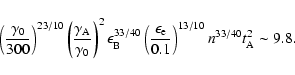
Combining Eqs. (12), (14) and (17), we get
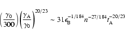 |
(18) |
 |
(19) |
Therefore Eqs. (12), (13) and (19) give the constraint on the parameters
 ,
,
 and n. Figure 2 shows the
relation between
,
and n. The
dotted, dash-dotted, dashed and dot-dot-dashed lines represent n=0.1,
1, 10 and 0.0016 respectively. We find that the allowed values of
and
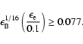
lie in the region confined by two lines Lc1 (Eq. (19)) and Lc2 (Eq. (13)). It is obvious that n must
be larger than 0.0016, and
must be larger than 0.0077. If we take n=1,
and n. Figure 2 shows the
relation between
,
and n. The
dotted, dash-dotted, dashed and dot-dot-dashed lines represent n=0.1,
1, 10 and 0.0016 respectively. We find that the allowed values of
and
lie in the region confined by two lines Lc1 (Eq. (19)) and Lc2 (Eq. (13)). It is obvious that n must
be larger than 0.0016, and
must be larger than 0.0077. If we take n=1,
 ,
then
,
then
 .
We propose that more observations are needed in
order to further estimate the values of
,
and n.
.
We propose that more observations are needed in
order to further estimate the values of
,
and n.
![\begin{figure}
\includegraphics[width=8cm,clip]{fa171_f1.eps}
\end{figure}](/articles/aa/full/2003/16/aafa171/Timg70.gif) |
Figure 1:
The optical light curve of
GRB 021211. The dashed line is the emission of the forward shock, the
dotted line represents the emission from reverse shock, and the solid
line is the total flux. Data from: Price & Fox (2002a, 2002b), Park et al. (2002), Li et al. (2002), Kinugasa et al. (2002), McLeod et al. (2002),
Wozniak et al. (2002), Levan et al. (2002). |
![\begin{figure}
\includegraphics[width=8cm,clip]{fa171_f2.eps}
\end{figure}](/articles/aa/full/2003/16/aafa171/Timg71.gif) |
Figure 2:
The relation between
,
and n given by Eqs. (12), (13)
and (19). The dotted, dash-dotted, dashed and dot-dot-dashed lines
represent n=0.1, 1, 10 and 0.0016 respectively. The allowed values of
and
lie in the region confined by
two lines Lc1 (Eq. (19)) and Lc2 (Eq. (13)). |
From Eq. (18) we see that the initial Lorentz factor  depends
on
and n very weakly, so as an approximation, and
taking
depends
on
and n very weakly, so as an approximation, and
taking
 ,
then we have
,
then we have
 .
Since the duration is about 15 s and the first
observation time is 65 s after the burst, so the value of
.
Since the duration is about 15 s and the first
observation time is 65 s after the burst, so the value of  should lie between 15 s and 65 s, and therefore we can get the initial
Lorentz factor
should lie between 15 s and 65 s, and therefore we can get the initial
Lorentz factor
 ,
which is consistent with the lower
limit estimates base on the
,
which is consistent with the lower
limit estimates base on the  - attenuation calculation
(Fenimore et al. 1993).
- attenuation calculation
(Fenimore et al. 1993).
Up: The afterglow of GRB 021211:
Copyright ESO 2003
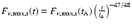
![$\displaystyle F_{\rm\nu,max,r}(t)\left
[\frac{\nu}{\nu_{\rm m,r}(t)}\right ]^{-(p-1)/2}$](/articles/aa/full/2003/16/aafa171/img63.gif)
![$\displaystyle F_{\rm\nu,max,r}(t_{\rm A})\left [\frac{\nu}{\nu_{\rm m,r}(t_{\rm...
... ]^{-\frac{(p-1)}{2}}\left(\frac{t}{t_{\rm A}}\right)^{-\frac{73p+21}{96}}\cdot$](/articles/aa/full/2003/16/aafa171/img64.gif)
![\begin{figure}
\includegraphics[width=8cm,clip]{fa171_f1.eps}
\end{figure}](/articles/aa/full/2003/16/aafa171/img70.gif)
![\begin{figure}
\includegraphics[width=8cm,clip]{fa171_f2.eps}
\end{figure}](/articles/aa/full/2003/16/aafa171/img71.gif)