A&A 402, 373-381 (2003)
DOI: 10.1051/0004-6361:20030027
Mars: Mapping surface units by means of statistical analysis
of TES spectra
F. Altieri 1 - G. Bellucci 1
CNR, Istituto di Fisica dello Spazio Interplanetario
00133 Rome, Italy
Received 28 November 2001 / Accepted 3 December 2002
Abstract
Thermal Emission Spectrometer (TES) data from the Mars
Global Surveyor (MGS) mapping phase have been processed to
identify regions with unique spectral features for new clues on
the Martian surface composition. For this purpose we have
developed a procedure to search and map band absorptions related
to presence of different surface minerals on a spatial scale of a
few kilometers. Data used in this study cover the March 1999-July 2000 period, corresponding to
 on Nili Fossae, Sinus Meridiani and
Valles Marineris regions, where outcrops of olivines and hematite have been
identified in previous studies. We have tested the validity of our
procedure on these areas and then extended our analysis to other
portions of the planet. The data have been assembled in
on Nili Fossae, Sinus Meridiani and
Valles Marineris regions, where outcrops of olivines and hematite have been
identified in previous studies. We have tested the validity of our
procedure on these areas and then extended our analysis to other
portions of the planet. The data have been assembled in
 emissivity spectra cubes with
 pixels per square degree. The Principal Components Analysis (PCA)
has been used to identify spectra with very low contamination by
atmospheric aerosols. It has been applied in two spectral ranges:
300-550 cm-1 (
pixels per square degree. The Principal Components Analysis (PCA)
has been used to identify spectra with very low contamination by
atmospheric aerosols. It has been applied in two spectral ranges:
300-550 cm-1 ( 18.2-33.3
  m) and 815-1143 cm-1 (8.7-12.3 m). By means of PCA we have
selected three principal spectral classes: spectra with a high
content of dust, spectra with a high content of water-ice and
spectra with a lower contamination by dust and water-ice. To
identify emission spectra with interesting features likely related
to surface minerals we have selected, in the last class, data with
high spectral variance between 300-550 cm-1, the range
where the hematite and olivine bands have been found.
m) and 815-1143 cm-1 (8.7-12.3 m). By means of PCA we have
selected three principal spectral classes: spectra with a high
content of dust, spectra with a high content of water-ice and
spectra with a lower contamination by dust and water-ice. To
identify emission spectra with interesting features likely related
to surface minerals we have selected, in the last class, data with
high spectral variance between 300-550 cm-1, the range
where the hematite and olivine bands have been found.
Key words: planets and satellites: individual: Mars -
techniques: spectrometric -
methods: data analysis
Over the last few years numerous attempts have been made to
determine the Martian surface and atmosphere composition to
understand the past geologic processes and past climates of the
planet. A large amount of data has been collected thanks to the
instruments aboard Mariner 6-7-9, Viking 1-2, and Phobos 2. Since
September 1997, the Mars Global Surveyor (MGS) NASA mission has
been orbiting around Mars and the Thermal Emission Spectrometer
(TES) has collected an enormous amount of data. The TES objectives
are (1) to determine and map the composition of surface minerals,
rocks and ices; (2) to study the composition, particle size and
spatial and temporal distribution of atmospheric dust; (3) to
locate water-ice and CO2 condensate clouds and determine their
temperature, height and condensate abundance; (4) to study the
growth, retreat and total energy balance of the polar cap
deposits; and (5) to measure the thermophysical proprieties of
Martian surface materials (Christensen et al. 1992). The MGS
spacecraft mapping phase began in March 1999 after the completion
of the aerobraking period. To date TES has acquired spectra over
an entire Martian year in a circular polar orbit with equator
crossing at 2 H and 14 H Mars local time (24 H equals one Martian
day). The interpretation of this huge quantity of data is
complicated by the difficulty of discriminating the different
contributions of surface and atmospheric components. One of the
principal scientific objective of the TES investigation is to
determine the composition of Martian surface. Included in its
spectral range are features caused by atmospheric components:
CO2 and water vapour gases,
dust and water ices aerosols. The measured spectrum is the result of emission,
absorption and transmission of energy by surface materials and by
atmospheric components. The surficial dust layer has a spectral
masking effect, generally smoothing the soil band contrast (Gaff
et al. 2001; Crisp & Bartholomew 1992). The main CO2 gas
absorption is centered at 667 cm-1 (15 m); other weaker
CO2 absorptions are centered at 550, 790, 961, 1064, 1260 and 1366 cm-1 (Maguire 1977). Dust aerosols have a principal
broad band centered at 1075 cm -1 and a minor broad band centered at 480 cm-1 (Huguenin 1987; Grassi & Formisano 2000). Water-ice
aerosols have a broad peak near 825 cm-1, a sharper peak at 229 cm-1 and minor absorption at wavenumbers >1000 cm-1, water vapour has absorption at 200-400 cm-1 and 1400-1800 cm-1 (Smith et al. 1999).
In this preliminary work we have developed a rapid method to
distinguish spectra strongly contaminated by atmospheric aerosols
(dust and ices), and to identify interesting surface spectral
features in one single TES detector spectrum. The method is
applicable to imaging spectrometry data gathered by future space
instrumentation as well. In Sect. 2 we describe briefly the TES
instrument characteristics, in Sect. 3 we describe the data used
in our study, in Sect. 4 we show the statistical method we have
used to select the spectra reported in Sect. 5 and, finally, in
Sect. 6 we draw some conclusions.
The Mars Global Surveyor Thermal Emission Spectrometer
consists of a Michelson interferometric spectrometer
collecting thermal infrared spectra between 6 and 50 m (200-1650 cm-1), with additional broadband visible (0.3-2.7 m) and thermal (5.5-100 m) channels (Christensen et al. 1992). Six detectors in a three-by-two array simultaneously
take infrared spectra with a selectable sampling of 5 or 10 cm-1 containing, respectively, 246 or 143 spectral channels.
The instantaneous field of view (IFOV) of each detector is 8.5 mrad corresponding to a spatial resolution of 3 km in
the final MGS mapping orbit altitude of 380 km. A pointing
mirror allows TES to carry out periodic view of an aboard
calibration blackbody and cold space, as well as measures in the
atmosphere above the limb. The TES noise equivalent spectral
radiance is
 W cm-2 sr-1 / cm-1 from 300 to 1400 cm-1, increasing to
 W cm-2 sr-1 / cm-1 at 250 cm-1 and
W cm-2 sr-1 / cm-1 at 1650 cm-1. Absolute radiometric accuracy has
been determined from pre-launch data to better than
W cm-2 sr-1 / cm-1 at 250 cm-1 and
W cm-2 sr-1 / cm-1 at 1650 cm-1. Absolute radiometric accuracy has
been determined from pre-launch data to better than
 W cm-2 sr-1 / cm-1 from 300 to 1400 cm-1 (Christensen et al. 1999; Christensen et al. 2000a;
Christensen et al. 2001). These random errors correspond to a
noise equivalent delta emissivity (NE
W cm-2 sr-1 / cm-1 from 300 to 1400 cm-1 (Christensen et al. 1999; Christensen et al. 2000a;
Christensen et al. 2001). These random errors correspond to a
noise equivalent delta emissivity (NE
 )
of 0.004 at 1000 cm-1 and 0.002 at 400 cm-1 for a surface
temperature of 275 K (Christensen et al. 2001b).
)
of 0.004 at 1000 cm-1 and 0.002 at 400 cm-1 for a surface
temperature of 275 K (Christensen et al. 2001b).
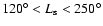
Data used in this study cover the period from March 1999 to July
2000, corresponding to an areocentric longitude of the Sun ( )
between 120
)
between 120 and 250.
We have initially selected
three regions: the first includes the region of Nili Fossae, where
the largest outcrop of olivine has been found (Hoefen et al. 2000;
Hoefen & Clark 2001; Hamilton et al. 2001); the others are on
Valles Marineris and Sinus Meridiani, two of the three regions
where TES team has identified outcrops of hematite (Christensen et al. 2001a; Lane et al. 2001; Christensen et al. 2000b). Then we
have extended our analysis to Sinai Planum, to a region between
Syrtis Major and northeastern Arabia Terra and to a portion of 60
and 250.
We have initially selected
three regions: the first includes the region of Nili Fossae, where
the largest outcrop of olivine has been found (Hoefen et al. 2000;
Hoefen & Clark 2001; Hamilton et al. 2001); the others are on
Valles Marineris and Sinus Meridiani, two of the three regions
where TES team has identified outcrops of hematite (Christensen et al. 2001a; Lane et al. 2001; Christensen et al. 2000b). Then we
have extended our analysis to Sinai Planum, to a region between
Syrtis Major and northeastern Arabia Terra and to a portion of 60
 on the Martian surface between 180
and 240 W and
on the Martian surface between 180
and 240 W and  and 30 N.
The data were collected during the MGS mapping phase, with a
constant orbit and a constant spatial resolution, so that they are
ideal to be visualized as cube images, having two spatial
dimensions and a third spectral dimension.
and 30 N.
The data were collected during the MGS mapping phase, with a
constant orbit and a constant spatial resolution, so that they are
ideal to be visualized as cube images, having two spatial
dimensions and a third spectral dimension.
The spectral calibrated radiance has been converted to emissivity
by (1) deriving the brightness temperature at each wavenumber; (2) assuming that the maximum of the brightness temperature around 1230 and 1300 cm-1 is the Christiansen peak (Christensen &
Harrison 1993; Ruff et al. 1997); (3) setting the maximum
brightness temperature equal to the surface kinetic temperature;
and (4) computing the emissivity at each wavenumber by dividing
the Planck function at the surface kinetic temperature
(Christensen et al. 2000b). The assumption that the surface
materials have unit emissivity at the point of maximum brightness
temperature for the thermal infrared emission has been
demonstrated to be valid to within 3% for a wide range of
minerals, rocks and soils (Salisbury et al. 1991; Ruff et al.
1997).
The emissivity spectra have been assembled in 10
 cubes with
pixels per square degree and
143 spectral channels. For all cubes we have considered 17 000 spectra with an emission angle between 30
and 60,
corresponding to a Martian local time of
cubes with
pixels per square degree and
143 spectral channels. For all cubes we have considered 17 000 spectra with an emission angle between 30
and 60,
corresponding to a Martian local time of
 and a mean surface temperature of 280 K.
All data have spectral sampling of 10 cm-1 and nadir view.
Because our aim was to obtain a good spatial coverage of the
examined regions, we have not constrained the data based on dust
and water-ice opacities.
and a mean surface temperature of 280 K.
All data have spectral sampling of 10 cm-1 and nadir view.
Because our aim was to obtain a good spatial coverage of the
examined regions, we have not constrained the data based on dust
and water-ice opacities.
Our aim was to find a procedure which allowed us: (1) to identify
the main spectral types responsible for the observed spectral
variation, and (2) identify regions or single TES pixels having
unique spectral contrast in the 300-500 cm-1 spectral
range. For this purpose, we have computed the Principal
Components Analysis (PCA) and the CHI-square error (CHISQR) of a
linear fit on some selected TES spectral channels. Combining these
two method of analysis we have been able to isolate spectra with
interesting features between 300 and 500 cm-1 spectral
domain.
PCA scatter plot. PCA is a technique commonly used in the
interpretation of terrestrial and spacecraft multispectral imaging
(Siegal & Gillespie 1980; Ardvison et al. 1982; Bell III et al.
1992). PCA involves the calculation of the eigenvectors of the
variance-covariance matrix of data set and then the transformation
of data onto a set of orthogonal axes that are linear combinations
of the original data (Davis 1986). The first axis, or Band 1,
contains the greatest amount of variance, with subsequent
components containing decreasing amount of variance. To avoid
water vapour and CO2 main features and TES wavenumbers where
the noise is higher, we have limited the PCA analysis to some
specific spectral channels and selected two main spectral ranges.
The first range is between 300 and 550 cm-1 (hereafter Range 1), where the hematite and olivine signatures have been found. For
the second range we have chosen spectral channels between 815 and 1143 cm-1 (hereafter Range 2), where the atmospheric aerosols
have deepest absorptions. We have found that (1) the PCA first
component (Band 1) in the Range 1 is well correlated with the
albedo (the correlation between the 20 m spectral channel and
the albedo was observed in Viking IRTM data as well (Christensen
1998)); and (2) the use of the second component (Band 2) in the
Range 1 and Range 2 to search for spectral variance related to
no-dust composition is the most convenient.
![\begin{figure}
\par\includegraphics[width=8.8cm,clip]{2140f1a.eps}
\end{figure}](/articles/aa/full/2003/16/aa2140/Timg22.gif) |
Figure 1:
a) PCA scatter plot of spectra from Nili Fossae region
cube. |
| Open with DEXTER |
![\begin{figure}
\par\includegraphics[width=8.8cm,clip]{2140f1b.eps}\end{figure}](/articles/aa/full/2003/16/aa2140/Timg25.gif) |
Figure 1:
b) Location of the spectral
classes on the albedo map. Spatial coverage
 N and N and
 W. Black pixels have no TES data in
the range used in this study. W. Black pixels have no TES data in
the range used in this study. |
| Open with DEXTER |
![\begin{figure}
\par\includegraphics[width=6cm,clip]{2140f1c.eps}
\end{figure}](/articles/aa/full/2003/16/aa2140/Timg26.gif) |
Figure 1:
c) Mean spectra of the classes reported in Fig. 1a. Cyan and blue spectra have typical features of water ice. The
red spectrum shows the principal dust band between 850 and 1200 cm-1 and the minor dust band between 300 and 550 cm-1.
Violet spectra are spread on albedo map dark regions while yellow
and green spectra are well grouped on the map and show the
olivine features. |
| Open with DEXTER |
The PCA algorithm has been applied to different
emissivity cubes showing similar results. In
this section we discuss the case of the Nili Fossae cube, where
Hoefen et al. (2000) have identified unique spectral features
related to olivine, and the Sinus Meridiani cube, where the
largest hematite outcrop has been found (Christensen et al.
2000b).
The south eastern corner of the Nili Fossae cube shows a local
maximum in emissivity at 451 and 377 cm-1 and a minimum at 408 cm-1. Using 5 cm-1 cm sampling spectra Hoefen et al.
(2000) have seen also a maximum at 303 cm-1 and a minimum at 292 cm-1 that are not well identifiable in our data because
of lower SNR in this spectral range and water vapour features.
They attributed these maxima to Christiansen peaks, with
similarities with sulfides and olivine. Figure 1a shows Range 1 - Range 2 PC2 Scatter Plot of the cube. The spatial coverage is of
N and
W. Each point on the scatter plot
corresponds to an emissivity spectrum of the cube. The spectral
units are identified on the scatter plot using different colors
and their position on the
albedo
map is reported below (Fig. 1b). This map has been assembled using
the TES broadband visible bolometer data. Dark pixels on the map
have no data in the period selected for our study. Mean
spectra of different spectral units are shown in Fig. 1c. Cyan and
blue spectra have typical features of water ice, they differ in
the dust content, higher in the cyan spectrum (Christensen et al.
2000b), and their locations on the scatter plot is in the region
where Range 2 PC2 have negative values. The red spectrum shows the
main dust band between 850 and 1200 cm-1 and the minor dust
band between 300 and 550 cm-1. Red spectra in the scatter
plot have Range 2 PC2 positive values, as well Range 1 PC2 values.
Violet spectra are spread on dark regions of the albedo map, while
yellow and green spectra are well grouped on the map and show the
olivine features. We can note how the red and blue spectra are
distributed on the typical three pixels TES narrow strips,
pointing out their dependence with
and atmospheric
conditions.
This method has been applied also to the Sinus Meridiani cube,
where the first and largest grey
hematite area has been identified by the TES team (Christensen et al.
2000b; Christensen et al. 2001a; Lane et al. 2001). Figure 2a shows
Range 1 - Range 2 PC2 scatter plot of the cube with a spatial
coverage of
 N and
N and
 W and the location of spectral classes are
reported on the albedo map in Fig. 2b. The mean spectra are shown
in Fig. 2c. Also in this case we can note how (1) the spectra with
dust are distributed in the region with Range 2 PC2 positive, (2) spectra with ice have Range 2 PC2 negative, (3) spectra with
surface features have near zero Range 2 PC2 and negative Range 1 PC2. Dark violet, violet, yellow and green spectra show different
percentage of dust (higher in the dark violet spectrum and minor
in the green one) and the same hematite signatures. They are
spatially grouped on the albedo map and seem to be aligned on a
straight line on the scatter plot. The red spectrum has a high
percentage of dust but does not have the surface hematite
features, in fact these spectra are distributed out of hematite
zone on the albedo map.
W and the location of spectral classes are
reported on the albedo map in Fig. 2b. The mean spectra are shown
in Fig. 2c. Also in this case we can note how (1) the spectra with
dust are distributed in the region with Range 2 PC2 positive, (2) spectra with ice have Range 2 PC2 negative, (3) spectra with
surface features have near zero Range 2 PC2 and negative Range 1 PC2. Dark violet, violet, yellow and green spectra show different
percentage of dust (higher in the dark violet spectrum and minor
in the green one) and the same hematite signatures. They are
spatially grouped on the albedo map and seem to be aligned on a
straight line on the scatter plot. The red spectrum has a high
percentage of dust but does not have the surface hematite
features, in fact these spectra are distributed out of hematite
zone on the albedo map.
The Range 1 - Range 2 PC2 scatter plot can be physically
interpreted as mappable features and spectral slope changes: dust
spectra with typical negative slopes in the 800-1100 cm-1 range have positive Range 2 PC2 values and spectra with positive
slopes in the 800-1100 cm-1 range, related to presence of
ice, have negative Range 2 PC2 values. Range 1 PC2 values are
related to the albedo as well: dark region spectra have Range 1 PC2 negative and bright region spectra have Range 1 PC2 values
near zero. This gives the scatter plot diagrams the typical form
of a boomerang. The length of the arms depends on the dust and ice
content in the atmosphere. High spectral variance related to
surface features has Range 1 PC2 values strongly negative and
Range 2 PC2 values near zero.
Although this method allows us to map the distribution of olivine
and hematite in these cubes, it does not work very well in the
case of spectral features related to smaller regions, as in the
case of the outcrop of hematite in Valles Marineris (Christensen
et al. 2001a). For this reason we have introduced the CHISQR
parameter.
CHISQR parameter. This is the CHI-square error in the linear fit of TES spectra
between 300 and 550 cm-1.
We have chosen this parameter because in this spectral range the effect of the dust is
to introduce a negative slope to the spectrum, if it is present in the atmosphere,
or to smooth spectral features, if it is deposited on the surface.
In both these cases the spectral range considered is well fitted
by a straight line with a more or less negative slope,
respectively, and CHISQR values will be small see (Fig. 3). On the
other hand, in the case of spectra with a high spectral variance
due to superficial
mineral absorptions, the linear fit will not be good, as well as in the case of spectra
with high ice content, having absorptions before 300 cm-1 and after 450 cm-1,
and CHISQR values will be high. In Fig. 3 we have reported mean
spectra from the cube centered on Candor Chasma and Ophir regions
where smaller outcrops of hematite have been identified
(Christensen et al. 2001a). The first spectrum from the top
presents higher content of dust than the other ones. The
absorption between 800 and 1200 cm-1 is deeper and the shape
of the spectrum between 300 and 550 cm-1 is characterized by
a smooth negative slope that is well reproduced by the linear fit
(small CHISQR value). The second spectrum presents a minor dust
content. The band absorption between 800 and 1200 cm-1 is lower, as well as the negative slope between 300 and 550 cm-1.
But again the spectrum in the last range is very smooth and the linear fit is good (small
CHISQR value). The third spectrum has a high content of water ice (deep absorption before 1000 cm-1 and minor absorptions before 300 cm-1 and after 450 cm-1).
The shape of the spectrum is not well reproduced by a straight line and the CHISQR value
is then higher than in the previous cases. The last spectrum is an average of the TES
pixels reported in Fig. 5. The hematite spectral signatures are
distinctly visible, and because of the presence of band
absorptions the spectrum is not smooth between 300 and 550 cm-1 and the CHISQR value is high. To distinguish between
spectra with high values of the CHISQR parameter but with a
different water ice content the PCA scatter plot can be used. In
conclusion, the CHISQR allows us to identify spectra with high
variance and the PCA allows us to discriminate within these
spectra the ones that have ice and the ones having features likely
related to surface. In Fig. 4 we have reported the Range 1 - Range 2 PC2 scatter plot for the Valles Marineris cube centered on Ophir
and Candor Chasma,
 S and
S and
 W.
We have marked with blue asterisks points with CHISQR > 0.002 and with red asterisks
the remaining points with high value for CHISQR related to
hematite spectra. Blue points are localized in the ice spectral
class, while red points are spread on the scatter plot. TES pixel
positions of some red asterix points are reported on MOC image
M0204452 (Malin et al. 2000) in Fig. 5, they are located on the
same Ophir region reported by Christensen et al. (2001a).
W.
We have marked with blue asterisks points with CHISQR > 0.002 and with red asterisks
the remaining points with high value for CHISQR related to
hematite spectra. Blue points are localized in the ice spectral
class, while red points are spread on the scatter plot. TES pixel
positions of some red asterix points are reported on MOC image
M0204452 (Malin et al. 2000) in Fig. 5, they are located on the
same Ophir region reported by Christensen et al. (2001a).
![\begin{figure}
\par\includegraphics[width=8.8cm,clip]{2140f2a.eps}
\end{figure}](/articles/aa/full/2003/16/aa2140/Timg31.gif) |
Figure 2:
a) PCA scatter plot of spectra from Sinus
Meridiani region cube. |
| Open with DEXTER |
![\begin{figure}
\par\includegraphics[width=8.8cm,clip]{2140f2b.eps}
\end{figure}](/articles/aa/full/2003/16/aa2140/Timg32.gif) |
Figure 2:
b) Location on the albedo map
of the spectral classes. Spatial coverage
N and
W. |
| Open with DEXTER |
![\begin{figure}
\par\includegraphics[width=6cm,clip]{2140f2c.eps}
\end{figure}](/articles/aa/full/2003/16/aa2140/Timg33.gif) |
Figure 2:
c) Mean spectra of the
classes reported in Fig. 2a. Blue and red spectra have water
ice and dust bands. The other spectra show a different percentage
of dust and the surface hematite features in the 300-500 cm-1 spectral range. |
| Open with DEXTER |
The other reason why we have computed the CHISQR is because it is
a more general parameter than the hematite index used by
Christensen et al. (2001a, 2000b) to identify TES pixels with
hematite. In fact, CHISQR is not defined by using some particular
TES spectral channels but is related to the entire 300-550 cm-1 spectral range, so that, by means of CHISQR, we have
been able to discriminate between both spectra with hematite and
olivine and spectra with features due to other minerals or mineral
mixtures, shown in the next section.
![\begin{figure}
\par\includegraphics[width=7.2cm,clip]{2140f3.eps}
\end{figure}](/articles/aa/full/2003/16/aa2140/Timg34.gif) |
Figure 3:
Mean spectra selected from the Candor Chasma
and Ophir cube. We have selected spectra with high dust content,
spectra with low dust content, spectra with high water ice content
and spectra with the signatures of hematite. For each one of these
spectral classes we have computed the linear fit between 300 and 550 cm-1 and the CHISQR values. The fit is reported with a
dashed line. From the plots it is evident how there is a good
correspondence between the linear fit and the first tow spectra
from the top (low values for CHISQR parameter), while in the case
of spectral classes with water ice and surface signatures the
spectral shape in the range selected is not so smooth (high
values for the CHISQR parameter). |
| Open with DEXTER |
![\begin{figure}
\par\includegraphics[width=8.8cm,clip]{2140f4.eps}
\end{figure}](/articles/aa/full/2003/16/aa2140/Timg35.gif) |
Figure 4:
PCA scatter plot for Candor Chasma and Ophir
cube. Spectra with CHISQR > 2 have been marked with a blue
asterisk. Spectra with hematite features have been marked with a
red asterisk. |
| Open with DEXTER |
![\begin{figure}
\par\includegraphics[width=8cm,clip]{2140f5.eps}
\end{figure}](/articles/aa/full/2003/16/aa2140/Timg37.gif) |
Figure 5:
MOC image M0204452 (Malin et al. 2000)
centered at
 and 4.70 S on the Ophir region
with the location of TES spectra showing the hematite features.
For the coordinate errors on MOC images, the position of TES
hematite spectra on the M0204452 image has been obtained combining
the spectra latitude and longitude values with the TES albedo
channel values.
and 4.70 S on the Ophir region
with the location of TES spectra showing the hematite features.
For the coordinate errors on MOC images, the position of TES
hematite spectra on the M0204452 image has been obtained combining
the spectra latitude and longitude values with the TES albedo
channel values. |
| Open with DEXTER |
![\begin{figure}
\par\includegraphics[width=8.8cm,clip]{2140f6.eps}
\end{figure}](/articles/aa/full/2003/16/aa2140/Timg38.gif) |
Figure 6:
Viking image with locations of the
TES pixels showing interesting features between 300 cm-1 and 500 cm-1. The bigger crater on the bottom is Baldet crater.
On the top right area of the image the final portion of Huo Hsing
Vallis is visible. White empty pixels have typical absorptions of
hematite spectra, black filled pixels show a band absorption at 360 cm-1 and black empty pixels have a band absorption at 390 cm-1. |
| Open with DEXTER |
![\begin{figure}
\par\includegraphics[width=8.25cm,clip]{2140f7a.eps}
\end{figure}](/articles/aa/full/2003/16/aa2140/Timg39.gif) |
Figure 7:
a) The first spectrum on the bottom is the
hematite mean spectrum from Sinum Meridiani. The Sp A spectrum is
the average of white empty TES pixels in Fig. 6. |
| Open with DEXTER |
![\begin{figure}
\par\includegraphics[width=8.25cm,clip]{2140f7b.eps}
\end{figure}](/articles/aa/full/2003/16/aa2140/Timg40.gif) |
Figure 7:
b) The first spectrum on the bottom is the mean
spectrum of the two black filled pixels in Fig. 6 having a band
absorption centered at 360 cm-1. The ASU Thermal
Emission Spectral Library magnetite sample (Christensen et al.
2000c) shows an absorption at the same wavenumber. |
| Open with DEXTER |
![\begin{figure}
\par\includegraphics[width=8.25cm,clip]{2140f7c.eps}
\end{figure}](/articles/aa/full/2003/16/aa2140/Timg41.gif) |
Figure 7:
c) Spectrum Sp C is the average of the black
empty pixels in Fig. 6 showing a band absorption centered at 390 cm-1. Spectra with similar features have been
identified spread over areas near Syrtis Major, Sp D, and on Sinai
Planum, Sp E. |
| Open with DEXTER |
Spectra with high values for the CHISQR parameter and low water
ice content have been found in northeastern Arabia Terra (
 W,
W,
 N). In Fig. 6 we have
reported a Viking image including the Baldet crater with the
superimposition of TES pixels showing significant variance in the
spectral range between 300 and 500 cm-1. White boxes in Fig. 6 show typical signatures of hematite. The mean spectrum is
labelled in Fig. 7a as Sp A. The mean spectrum of the Sinus
Meridiani hematite spectra is indicated as SM and has been plotted
for comparison. The hematite index value for the SM mean spectrum
is 1.028 and for the Sp A spectrum is 1.015. The detection limit
for the hematite band indicated in Christensen et al. (2001a) is 1.018, and the hematite index value found for the vast majority of
TES spectra is 1.010, with a variation of
N). In Fig. 6 we have
reported a Viking image including the Baldet crater with the
superimposition of TES pixels showing significant variance in the
spectral range between 300 and 500 cm-1. White boxes in Fig. 6 show typical signatures of hematite. The mean spectrum is
labelled in Fig. 7a as Sp A. The mean spectrum of the Sinus
Meridiani hematite spectra is indicated as SM and has been plotted
for comparison. The hematite index value for the SM mean spectrum
is 1.028 and for the Sp A spectrum is 1.015. The detection limit
for the hematite band indicated in Christensen et al. (2001a) is 1.018, and the hematite index value found for the vast majority of
TES spectra is 1.010, with a variation of  0.002 consistent with instrumental noise. As reported in Christensen et al. (2000a) high values of the hematite index can be found also
for spectra with significant water ice opacity. This implies that
the mean value of the hematite index increases if any selection is
done in the TES spectra and if data with a high content of water
ice are included. Choosing spectra close to the area mapped in
Fig. 6 and with low ice content and no hematite signatures, we
have found a hematite index value for TES data of 1.004,
and the value of 1.015 could be considered acceptable. The
different band contrast at 300 cm-1 of Sp A compared
with SM spectrum could be due to a different hematite abundance
and the different shape of the maximum at 500 cm-1could be due to the presence of other mixed materials (Morris et al. 2001) or of a surface dust coating that masks their real
abundance (Gaff et al. 2001; Crisp & Bartholomew 1992). The
average of the two spectra with black filled pixels is reported in
Fig. 7b as Sp B. A band absorption centered at 360 cm-1 is clearly visible and is perhaps due to magnetite. The
band depth, in percent, of the TES 360 cm-1 feature is 2.1,
while the band detection limit on the same spectral region
computed by Kirkland et al. (2001) for TES is of the order of 1.4, assuming a confidence factor of 2 for the peak to peak
noise and a target band full width at the half of the maximum of
the band depth of 30 cm-1. In Fig. 7c we have reported the
mean spectrum of the dark empty pixels as Sp C. A band centered at 390 cm-1 is visible as well as in Sp D and Sp E,
identified in different areas, respectively near Syrtis Major and
on Sinai Planum. The band depth for Sp C is 1.9, for Sp D is 2.3
and for Sp E is 1.5. The majority of the spectra mapped in Fig. 6
come from the same TES orbit and are located near Huo Hsing
Vallis. This region presents a heavily cratered terrain,
characterized by a mantling deposit of horizontally layered
material subsequently subjected to erosion (Moore 1990). Erosion
of this extent suggests that the material is easily broken down
into transportable elements. Speculative origins for the deposit
include formation as differently welded pyroclastic tuff or a
compacted aeolian dust deposit. The hypothesis that the deposit
could have an underformed, horizontal, massive, water-laid
sedimentary origin has been discarded by Moore (1990) due to the
lack of compelling fluvial or lacustrine geomorphic features on
the Mars highlands. The understanding of all minerals responsible
for the observed bands in the 300-550 cm-1 TES spectral
range could give us new clues about the past history and formation
of this region of the planet.
0.002 consistent with instrumental noise. As reported in Christensen et al. (2000a) high values of the hematite index can be found also
for spectra with significant water ice opacity. This implies that
the mean value of the hematite index increases if any selection is
done in the TES spectra and if data with a high content of water
ice are included. Choosing spectra close to the area mapped in
Fig. 6 and with low ice content and no hematite signatures, we
have found a hematite index value for TES data of 1.004,
and the value of 1.015 could be considered acceptable. The
different band contrast at 300 cm-1 of Sp A compared
with SM spectrum could be due to a different hematite abundance
and the different shape of the maximum at 500 cm-1could be due to the presence of other mixed materials (Morris et al. 2001) or of a surface dust coating that masks their real
abundance (Gaff et al. 2001; Crisp & Bartholomew 1992). The
average of the two spectra with black filled pixels is reported in
Fig. 7b as Sp B. A band absorption centered at 360 cm-1 is clearly visible and is perhaps due to magnetite. The
band depth, in percent, of the TES 360 cm-1 feature is 2.1,
while the band detection limit on the same spectral region
computed by Kirkland et al. (2001) for TES is of the order of 1.4, assuming a confidence factor of 2 for the peak to peak
noise and a target band full width at the half of the maximum of
the band depth of 30 cm-1. In Fig. 7c we have reported the
mean spectrum of the dark empty pixels as Sp C. A band centered at 390 cm-1 is visible as well as in Sp D and Sp E,
identified in different areas, respectively near Syrtis Major and
on Sinai Planum. The band depth for Sp C is 1.9, for Sp D is 2.3
and for Sp E is 1.5. The majority of the spectra mapped in Fig. 6
come from the same TES orbit and are located near Huo Hsing
Vallis. This region presents a heavily cratered terrain,
characterized by a mantling deposit of horizontally layered
material subsequently subjected to erosion (Moore 1990). Erosion
of this extent suggests that the material is easily broken down
into transportable elements. Speculative origins for the deposit
include formation as differently welded pyroclastic tuff or a
compacted aeolian dust deposit. The hypothesis that the deposit
could have an underformed, horizontal, massive, water-laid
sedimentary origin has been discarded by Moore (1990) due to the
lack of compelling fluvial or lacustrine geomorphic features on
the Mars highlands. The understanding of all minerals responsible
for the observed bands in the 300-550 cm-1 TES spectral
range could give us new clues about the past history and formation
of this region of the planet.
![\begin{figure}
\par\includegraphics[width=8cm,clip]{2140f8.eps}
\end{figure}](/articles/aa/full/2003/16/aa2140/Timg45.gif) |
Figure 8:
Mean TES spectrum having a broad absorption
between 300 and 500 cm-1. |
| Open with DEXTER |
![\begin{figure}
\par\includegraphics[width=8cm,clip]{2140f9.eps}
\end{figure}](/articles/aa/full/2003/16/aa2140/Timg46.gif) |
Figure 9:
The Sinai Pl. spectrum is the average of six
adjacent TES pixels from Sinai Planum, the Aeolis Hg. spectrum is
the average of five adjacent pixels collected on a region near Aeolis Highland.
These two spectra acquired at different longitudes
show same signatures at 340, 410 cm-1 and 490 cm-1. |
| Open with DEXTER |
In Fig. 8 we have reported the mean of fifteen single TES spectra
coming from adjacent sensors and acquired on areas centered at 215.3 W and 13.6 N, 222.6 W and 0.1 N, 238.6 W and 18.0 S. A broad band
absorption centered at 400 cm-1 is clearly visible.
In Fig. 9 the average of five TES spectra from Aeolis Highland
(Aeolis Hg.) and six TES spectra from Sinai Planum (Sinai Pl.) are
reported. Although they have been collected at different
longitudes, they show similar signatures: absorptions at 340 and 490 cm-1 and a maximum at 410 cm-1. We have not computed the band depth for these spectra
since it is not clear where to assume the continuum lies. In fact
the band at 490 cm-1 is cut on the right by CO2absorptions and the band at 340 cm-1 is on the left border of
the TES spectral range.
As the principal purpose of this study is the description of the
spectral statistical analysis applicable for mapping the surface
of Mars, a best understanding of the new spectral features
observed between 300 cm-1 and 500 cm-1 and shown in this
section is reserved for future works, as is as the discussion
about other absorptions present between 800 cm-1 and 1300 cm-1. Only the library spectrum of magnetite has been
reported due to the evident similarity between the laboratory and
the TES spectra. Magnetite has been suggested as a component of
magnetic material found in Martian soil (Hargraves et al. 1979;
Pollack et al. 1977)
and has been identified in some Martian meteorites (Scott 1999).
Although the number of spectra reported in this study is small
compared to the huge
amount of data collected by TES, they show between 300 cm-1and 500 cm-1 features that could give new information about
Martian surface properties.
We want to stress here the fact that, except for rare exceptions,
the Martian surface does not show strong spectral variations at
spatial scales  10 km in the 300-500 cm-1 spectral
range. This suggests that only spectral analysis at higher spatial
resolution can give new clues on Martian mineralogy. Clays and
carbonates are expected to exist on Mars if water was abundant in
the past (Pollack et al. 1987; Catling 1999). A failure in
detection of these minerals could be due to the fact that they
occur in small patches (areal coverage
10 km in the 300-500 cm-1 spectral
range. This suggests that only spectral analysis at higher spatial
resolution can give new clues on Martian mineralogy. Clays and
carbonates are expected to exist on Mars if water was abundant in
the past (Pollack et al. 1987; Catling 1999). A failure in
detection of these minerals could be due to the fact that they
occur in small patches (areal coverage  10 km2) on the
Martian surface and in low concentrations. This was the main
reason why we developed a method to identify single TES spectra
(spatial footprint
10 km2) on the
Martian surface and in low concentrations. This was the main
reason why we developed a method to identify single TES spectra
(spatial footprint
 km).
km).
There are two principal conclusions that we can draw from this
study. The first one is that the combined use of a Range 1 - Range 2 PC2 scatter plot with the CHISQR parameter allows us to
identify single TES data with high spectral variance in the 300-500 cm-1 range attributable to superficial components. The
Range 1-Range 2 PC2 scatter plot characterizes in each cube
spectral classes having similar dust content, similar ice content
or similar superficial features. If data with interesting 300-500 cm-1 spectral features are limited and spread on the
Martian surface, then the use of the CHISQR parameter is
necessary. In this way we have been able to identify hematite
outcrops in Valles Marineris, already studied by the TES team, and
new unique spectra in a region between northeastern Arabia Terra
and Syrtis Major, in Sinai Planum, and spread over a region
between west Elysium Planitia and Terra Cimmeria. The fact that
these bands have characteristics distinct from those observed in
the atmospheric bands lets us suppose that they can be caused by
the surface components, as in the case of hematite.
The second conclusion is that on the Martian surface there are
spots with a dimension of 3-10 km whose spectra show
absorption bands between 300 and 500 cm-1 never observed in
previous studies. The signatures they show recur at some specific
wavenumbers, so that these bands could be related to some specific
mineralogical typologies. If these observed spots are outcrops of
the same dimension of the order of 3-10 km, or if they
are larger but spectrally obscured by a surface dust coating is
not still clear. The interpretation of these spectra in terms of
possible mineralogy will be the object of a future study.
Acknowledgements
Authors wish to thank Mrs S. Zampieri and Dr. L. Di Fino for the help in the
manuscript preparation and Dr Scott Nowicki for the careful review of the paper.
Funding were provided by ASI grants.
- Arvidson, R. E., Guinness, E. A., & Zent, A. P. 1982,
J. Geophys. Res., 87, 10149
- Bell, J. F. III, Lucey, P. G., & McCord, T. B. 1992,
Experimental Astronomy, 2, 287
In the text
- Catling, D. C. 1999,
J. Geophys. Res., 104, 16453
In the text
- Christensen, P. R., Anderson, D. L.,
Stillman, C. C., et al. 1992,
J. Geophys. Res., 97, 7719
In the text
NASA ADS
-
Christensen, P. R., & Harrison, S. T. 1993,
J. Geophys. Res., 98 (B11), 19819
In the text
- Christensen, P. R. 1997,
J. Geophys. Res., 103, 1733
- Christensen, P. R. 1999,
Calibration Report for the Thermal Emission Spectrometer (TES)
for the Mars Global Surveyor Mission, Mars Global Surveyor Project,
Jet Propul. Lab., Pasadena, Calif.
In the text
- Christensen, P. R., Bandfield, J. L.,
Smith, M. D., et al. 2000a,
J. Geophys. Res., 105, 9609
In the text
NASA ADS
- Christensen, P. R., Bandfield, J. L.,
Clark, R. N., et al. 2000b,
J. Geophys. Res., 105, 9623
In the text
NASA ADS
- Christensen, P.R., Bandfield, J. L.,
Hamilton, V. E., et al. 2000,
J. Geophys. Res., 105, 9735
NASA ADS
- Christensen, P. R., Morris, R. V.,
Lane, M. D., et al. 2001a, J. Geophys. Res., 106, 22873
In the text
- Christensen, P. R., Bandfield, J. L.,
Hamilton, V. E., et al. 2001b,
J. Geophys. Res., 106, 23823
In the text
- Crisp, J., & Bartholomew, M. J. 1992,
J. Geophys. Res., 97, 14691
In the text
- Davis, J. C. 1986,
in Statistics and Data Analysis in Geology (New York:
John Wiley and Sons Pubs.), 527
In the text
- Graff, T. G., Morris, R. V., & Christensen, P. R. 2001,
Effects of Palagonitic Dust Coatings on Thermal Emission Spectra
of Rocks and Minerals: Implications for Mineralogical
characterization of the Martian Surface by MGS-TES,
Lunar and Planet. Sci [CD-ROM], XXXII, Abstract 1899
- Grassi, D., & Formisano, V. 2000,
Planet. Space Sci., 48, 577
In the text
NASA ADS
- Hamilton, V. E., Christensen, P. R., & McSween, H. Y. 2001,
Spectral variations in MGS TES Data of Nili Fossae: A possible
source region for SNC Meteorites on Mars?,
Lunar and Planet. Sci. [CD-ROM], XXXII, Abstract 2184
In the text
- Hargraves, R. B., Collinson, D. W., Arvidson, R. E., & Cates, P. M. 1979,
J. Geophys. Res., 84, 8379
In the text
NASA ADS
- Hoefen, T. M., & Clark, R. N. 2001,
Compositional Variability of Martian Olivines Using Mars
Global Surveyor Thermal Emission Spectra,
Lunar and Planet. Sci [CD-ROM], XXXII, Abstract 2049
In the text
- Hoefen, T. M., Clark, R. N., Pearl, J. C., et al. 2000,
Unique Spectral features in Mars Global Surveyor Thermal
Emission Spectrometer: Implication for Surface Mineralogy in Nili Fossae,
American Astronomical Society, DPS meeting, 32, 62.03
In the text
- Huguenin, R. L. 1987,
Icarus, 10, 162
In the text
- Kirkland, L. E., Herr, K. C., Salisbury, J. W., et al. 2001,
Detecting Minerals on Mars using TES, THEMIS, and min-TES,
Workshop on the Martian Highlands and Mojave Desert Analogs (2001), Abstract 4025
In the text
- Lane, M. D., Hartmann, W. K., Berman, D. C., et al. 2001,
Update on studies of Martian hematite-rich areas,
Lunar and Planet. Sci. [CD-ROM], XXXII, Abstract 1984
In the text
- Maguire, W. C. 1977,
Icarus, 32, 85
In the text
NASA ADS
- Malin, M. C., Edgett, K. S., Davis, S. D.,
et al. 2000, M02-04452, Malin Space Science Systems Mars
Orbiter Camera Image Gallery ( In the text
http://www.msss.com/moc_gallery/), 22 May 2000
- Moore, J. M. 1990,
J. Geophys. Res., 95, 14279
In the text
- Morris, R. V., Lane, M. D., Mertzman, S., Shelfer, T.
D., & Christensen, P. R. 2001, Chemical and Mineralogical Purity of
Sinus Meridiani
Hematite, Lunar and Planet. Sci [CD-ROM], XXXI, Abstract 1618
In the text
- Pollack, J. B., Colburn, D., Kahn, R., et al.
1977,
J. Geophys. Res., 82, 4479
In the text
NASA ADS
- Pollack, J. B., Kasting, J. F., Richardson, S. M., et al.
1987,
Icarus, 71, 203-224
In the text
- Ruff, S. W., Christensen, P. R., Barbera, P. W., et al. 1997,
J. Geophys. Res., 102, 14899
In the text
- Salisbury, J. W., & Walker, L. W. 1989,
J. Geophys. Res., 94, 9192
NASA ADS
- Salisbury, J. W., Walter, L. S., Vergo, N., et al. 1991,
in Infrared (2.1-25 m) Spectra of Minerals, 267 pp. (Baltimore, Md.:
Johns Hopkins Univ. Press)
In the text
- Scott, E. R. 1999,
J. Geophys. Res., 104, 3803
In the text
NASA ADS
- Siegal, B. S., & Gillespie, A. R. 1980,
Remote Sensing in Geology,
(New York: John Wiley and Sons Pubs.), 200 pp.
In the text
- Smith, M. D., Christensen, P. R., & Bandfield, J. L. 1999,
J. Geophys. Res., 105, 9589
In the text
Copyright ESO 2003
![\begin{figure}
\par\includegraphics[width=8.8cm,clip]{2140f1a.eps}
\end{figure}](/articles/aa/full/2003/16/aa2140/img22.gif)
![\begin{figure}
\par\includegraphics[width=8.8cm,clip]{2140f1b.eps}\end{figure}](/articles/aa/full/2003/16/aa2140/img25.gif)
![\begin{figure}
\par\includegraphics[width=6cm,clip]{2140f1c.eps}
\end{figure}](/articles/aa/full/2003/16/aa2140/img26.gif)
![\begin{figure}
\par\includegraphics[width=8.8cm,clip]{2140f2a.eps}
\end{figure}](/articles/aa/full/2003/16/aa2140/img31.gif)
![\begin{figure}
\par\includegraphics[width=8.8cm,clip]{2140f2b.eps}
\end{figure}](/articles/aa/full/2003/16/aa2140/img32.gif)
![\begin{figure}
\par\includegraphics[width=6cm,clip]{2140f2c.eps}
\end{figure}](/articles/aa/full/2003/16/aa2140/img33.gif)
![\begin{figure}
\par\includegraphics[width=7.2cm,clip]{2140f3.eps}
\end{figure}](/articles/aa/full/2003/16/aa2140/img34.gif)
![\begin{figure}
\par\includegraphics[width=8.8cm,clip]{2140f4.eps}
\end{figure}](/articles/aa/full/2003/16/aa2140/img35.gif)
![\begin{figure}
\par\includegraphics[width=8cm,clip]{2140f5.eps}
\end{figure}](/articles/aa/full/2003/16/aa2140/img37.gif)
![\begin{figure}
\par\includegraphics[width=8.8cm,clip]{2140f6.eps}
\end{figure}](/articles/aa/full/2003/16/aa2140/img38.gif)
![\begin{figure}
\par\includegraphics[width=8.25cm,clip]{2140f7a.eps}
\end{figure}](/articles/aa/full/2003/16/aa2140/img39.gif)
![\begin{figure}
\par\includegraphics[width=8.25cm,clip]{2140f7b.eps}
\end{figure}](/articles/aa/full/2003/16/aa2140/img40.gif)
![\begin{figure}
\par\includegraphics[width=8.25cm,clip]{2140f7c.eps}
\end{figure}](/articles/aa/full/2003/16/aa2140/img41.gif)
![\begin{figure}
\par\includegraphics[width=8cm,clip]{2140f8.eps}
\end{figure}](/articles/aa/full/2003/16/aa2140/img45.gif)
![\begin{figure}
\par\includegraphics[width=8cm,clip]{2140f9.eps}
\end{figure}](/articles/aa/full/2003/16/aa2140/img46.gif)