A&A 401, 1159-1175 (2003)
DOI: 10.1051/0004-6361:20030214

Astrometric reduction of lightcurves observed during the PHESAT95 campaign of Saturnian satellites

B. Noyelles^1,2 - A. Vienne^1,2 - P. Descamps¹

1 - Institut de mécanique céleste et de calcul des éphémérides - Observatoire de Paris, UMR 8028 du CNRS, 77 avenue Denfert-Rochereau, 75014 Paris, France
2 - Université de Lille, 59000 Lille, France

Received 19 November 2002 / Accepted 17 January 2003

Abstract
In this paper, we present astrometric results derived from reduction of 65 lightcurves made in 1995-1996 during the PHESAT95 campaign of observation of Saturnian satellites mutual events. These results have an accuracy of about 20-30 mas and are compared to those obtained by Emelianov et al. (1997) for the 3 events observed in Crimea and Kazakhstan. We also discuss the reliability of the method used for reducing the lightcurves from the mutual events of 1980.

Key words: planets and satellites: individual: Saturn - astrometry

1 Introduction

Since the 1970s the IMCCE has carried out systematic campaigns of observations of mutual events of Jovian and Saturnian satellites. In the case of Saturnian satellites, mutual events are visible about every 15 years, when the Earth and the Sun cross the rings' plane. This was the case in 1995, so mutual events were observed during this period as predicted by Arlot & Thuillot (1993) and observations were published by Thuillot et al. (2001) under the name PHESAT95. The PHESAT95 campaign consists of 65 lightcurves obtained by an international network of 16 observation sites involving satellites S-1 Mimas, S-2 Enceladus, S-3 Tethys, S-4 Dione, S-5 Rhea and S-6 Titan. This paper aims to give astrometrical coordinates obtained after reduction of these lightcurves and to compare our method with others used before, to discuss the reliability of these works. The astrometric reduction of these lightcurves could be useful in improving the TASS1.6 theory (Vienne & Duriez 1995) and in the interpretation of the observations that will be made by the CASSINI space probe in the Saturnian system.

2 The theoretical lightcurves

2.1 Modeling a mutual event

It is necessary to model the mutual events before reducing their lightcurves. Let us first describe an occultation.

2.1.1 Modeling an occultation

An occultation between two solar system bodies consists of one of these bodies being at least partially hidden by the other one, in such a way that the observer cannot see two disks separately, since he is nearly aligned with the centres of the two satellites involved. Before and after the event, the observer detects the solar light reflected by the two satellites, whereas during the event the light reflected by the further satellite is partially hidden by the other one. Consequently, the observer registers a light flux drop.

Since modeling an occultation requires one to predict it, we used TASS1.6 (Vienne & Duriez 1995) for the satellites and SLP96 (using Chebychev's coefficients deduced from the VSOP87 theory, Bretagnon & Francou 1988) after correcting light travel time. The light-time correction consists of two iterations, the first one evaluating the light-time between Saturn and the observer at the observation date, the second one evaluating the light time between the observer and the centre of each satellite (observation time - first light time calculated), taking account of the light travel time between the two satellites. We took into account the refraction and the annual aberration too, these effects altering the results by less than 1 mas.

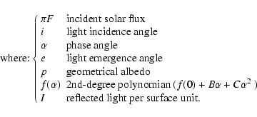
In order to determine the light flux detected by the observer, we considered each satellite as a sphere composed of multiples facettes (at least 10 000 to see reliable theoretical lightcurves, in fact more than 60 000 were required to have an "acceptable'' convergence efficiency when fitting the model to the observed lightcurve). On each sphere we have associated a reference frame (x, y, z) centered on the centre of the satellite whose x-axis pointed to the observer, the (x, z) plane being defined by the directions satellite-observer ($\vec{x}$) and satellite-sun, while $\vec{y}$ completed the direct trihedron. Then, we used two angles, $\lambda$ and $\phi$, $\lambda$ varying between  $-90^{\circ}$ and  $90^{\circ}-{\alpha}$ where ${\alpha}$ is the phase angle, and $\phi$ varying between  $-90^{\circ}$ and  $90^{\circ}$ (see Fig. 1).

	Figure 1: Orientation of satellite.
Open with DEXTER

   

Table 1: Values of the photometric parameters used for the five first satellites, from Buratti & Veverka (1984) and Devyatkin & Miroshnichenko (2001).

satellite	A	f(0)	B	C
S-1	0.7	1.1	-0.86	0.19
S-2	0.4	2.4	-0.51	-0.17
S-3	0.7	1.45	-0.95	0.20
S-4	1.0	1.0	-1.24	0.50
S-5	0.95	1.1	-1.33	0.54

This representation of a satellite is useful to apply a light scattering law. The most used laws are the Lambert law for a body with an atmosphere and the Minnaert and Hapke laws for other bodies, but these last two laws depend on photometric parameters that are not well determined for Saturnian satellites. We finally decided to use the Lambert law for Titan, because this body has an atmosphere and its geometrical albedo is well known (see Neff et al. 1984 for its values depending on the wavelength). A law issued from the Lommel-Seeliger law was used by Devyatkin & Miroshnichenko (2001) for the five other satellites using numerical parameters published by Buratti & Veverka (1984) (see Table 1 for the numerical values; we used respectively 196.2, 247.3, 528.2, 560, 764 and 2575 km for the radii). The mathematical formulae we used are

$$\frac{I}{F}=A\frac{\cos(i)}{\cos(i)+\cos(e)}f(\alpha)+(1-A)\cos(i)$$ (1)

for the first five satellites and

$$\frac{I}{F}=\frac{3}{2}p\cos(i)$$ (2)

for Titan (isotropic scattering)

$$\textrm{where:} \left \{ \begin{array} {ll}{\pi}F & \textrm{i... ...\textrm{reflected light per surface unit.} \end{array} \right.$$

The total light flux is thus deduced after numerical quadrature (see Descamps 1992 for further details).

2.1.2 Modeling an eclipse

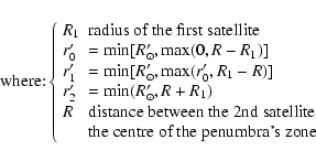
An eclipse corresponds to a near alignment between the Sun and two Saturnian satellites, one of them eclipsing the other one. It may be seen from the second satellite as an occultation of the Sun by the first one. Its representation is nearly the same as for an occultation. The main difference between the observation of the two kinds of event is the penumbra zone, where the solar light is only partially hidden (see Fig. 2).

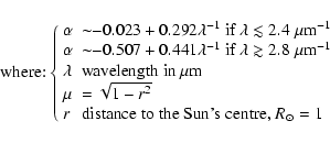
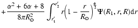
For modeling the light intensity in the penumbra zone, we took the Sun's limb darkening into account. We modeled the Sun's light flux by using the following law (Hestroffer & Magnan 1998):

$$I(\mu)={\mu}^{\alpha}$$ (3)

$$\textrm{where:} \left \{ \begin{array} {ll}{\alpha} & {\sim}{... ...istance to the Sun's centre, } R_{\odot}=1 \end{array} \right.$$

and thus calculated the solar flux $i_{\odot}$ received by each point of the eclipsed satellite in the penumbra zone, that is required to integrate Eq. (3) over the solar disk. For this purpose, we obtained the following formula, inspired by Aksnes' calculation (Aksnes & Franklin 1976) but with another formula for the Sun's limb darkening (r being now in AU):

 

$$i_{\odot} 1-\frac{1}{2R_{\odot}^2}\bigg[\Big(1-\frac{r}{R_{\odot}}\Big)^{\frac{\alpha}{2}} (r-R_{\odot})(2(r+R_{\odot})+{\alpha}r)\bigg]^{r'_1}_{r'_0}$$ =

$$+\frac{\alpha^2+6\alpha+8}{8{\pi}R_{\odot}^{2}}\int_{r'_1}^{r'_2}r \Big(1-\frac{r}{R_{\odot}}\Big)^\frac{\alpha}{2}\Psi(R_1,r,R){\rm d}r$$ (4)

$$\textrm{where:} \left \{ \begin{array} {ll}R_1 & \textrm{radi... ...\textrm{the centre of the penumbra's zone} \end{array} \right.$$

$R'_{\odot}$ is the Sun's radius seen from the 2nd satellite, as if the Sun and the 1st satellite were at the same distance, and $\Psi$ is defined by:

$$\Psi(R_1,r,R)=2\arctan\Bigg(\frac{\sqrt{r^2-a^2}}{a}\Bigg)$$ (5)

where

$$a=\frac{r^2+R^2-R_1^2}{2R}\cdot$$ (6)

Another difference between an eclipse and an occultation is that the light loss is not due to light reflected by the second satellite not seen by the observer, but to light not reflected by the second satellite. This is why when we calculate the light travel time, we have to consider where the first satellite was when it blocked solar light during its travel to the second satellite, whereas for an occultation we had to consider the time when the first satellite reflected solar light (see Fig. 3). More precisely, the light time correction for the first satellite is $t_{d_2}+t_{\Delta}$ in the case of an eclipse whereas it is $t_{d_1}({\approx}t_{d_2}-t_{\Delta})$ in the case of an occultation (Arlot 1985). The difference between both light times is usually between one and three seconds. For most of the eclipses, the eclipsing satellite is involved in the photometric measurement, which has required to calculate t_d1 too.

	Figure 2: Geometry of an eclipse.
Open with DEXTER

	Figure 3: Light time correction for an eclipse.
Open with DEXTER

The next step of the modelization is not very different from the calculus made in the case of an occultation, Eq. (4) being used in Eqs. (1) and (2) for the numerical quadrature over the eclipsed satellite.

   

Table 2: A result with and without velocity adjusted (2o1 means that S2 occults S1).

Event	midtime	impact (km)	velocity (km s-1)
2o1,8/16	3 45 22	119.3	3.38
OHP	$\sigma$ 4.8 s	$\sigma$ 15.2	$\sigma$ $7.8\times 10^{-2}$
	3 45 17	0	14.56
	$\sigma$ 0.4 s	$\sigma$ 1.1

2.2 Obtained lightcurves

Figure 4 shows a mutual event represented by the method described above. The x-axis indicates the decimal hour and the y-axis indicates the normalized flux ( $\rm flux=1$ means that the two satellites are theoretically completely visible separately). As a comparison we give the measures made during this event converted into relative flux (see Fig. 5), to check that our model gives something "reliable'', at least by its shape.

	Figure 4: Theoretical lightcurve of an occultation of Tethys by Dione seen at the Pic du Midi observatory on September 21st, 1995. The axes show the decimal hour (UTC) horizontally and the normalized light vertically. The axes will be the same for each lightcurve in this paper.
Open with DEXTER

	Figure 5: Measures of flux drop made at the Pic du Midi observatory during the occultation of Tethys by Dione on September 21st, 1995. This lightcurve could be compared with the theoretical lightcurve Fig. 4 when looking at its shape, but when keeping in mind that the theoretical lightcurve is not fitted to the measures. Figure A.1 shows the fitted model and the measure on the same picture.
Open with DEXTER

Two quantities derived from the lightcurve are to be noticed: the midlight time and the flux drop. The midlight time is the time when the satellites' magnitude is the least, whereas the flux drop corresponds to the least visible light flux; it is the flux corresponding to the midlight time. It seems clear that the midlight time corresponds to the time when the two satellites are closest on the celestial sphere (we call it midtime), in fact these two times are separated by a few seconds because of light scattering by the surface of atmosphereless satellites and the phase effect (see for example Aksnes 1986). The light flux drop can be directly linked to what we call the impact parameter, which is the distance between the centre of the first satellite (that nearer the observer) and the line joining the observer to the centre of the second satellite (in the case of an eclipse, the impact parameter is seen from the Sun's centre).

 

 

Table 3: Results obtained after reduction of the PHESAT95 lightcurves (2e3 means that S2 eclipses S3, and 3eo2 means that both an eclipse and an occultation of Enceladus by Tethys were predicted during the observation).

Event	midtime	impact parameter
	(hms)	(km)
2e3,6/17	1 56 46	199.9
OHP	$\sigma$ 0.5 s	$\sigma$ 3.5
3e2,7/22	0 04 36	53.9
OHP	$\sigma$ 2.9 s	$\sigma$ 126.2
3e2,7/22	0 03 52	294.3
Catania	$\sigma$ 1.3 s	$\sigma$ 7.3
3e2,7/22	0 04 25	571.9
Pic du Midi	$\sigma$ 2 s	$\sigma$ 3.6
4e3,7/28	9 23 01	771.6
ESO	$\sigma$ 1.5 s	$\sigma$ 3.1
2o3,7/29	1 05 39	0
Catania	$\sigma$ 9.6 s	$\sigma$ 0.46
3e1,8/2	9 45 04	2.3
ESO	$\sigma$ 4.1 s	$\sigma$ $5.6\times 10^{7}$
3e1,8/4	7 03 38	683
ESO	$\sigma$ 17.6 s	$\sigma$ 38.1
5o4,8/6	21 34 14	0.1
Catania	$\sigma$ 0.7 s	$\sigma$ 52
5o4,8/6	21 34 47	952
Crimea	$\sigma$ 0.8 s	$\sigma$ 5.2
3e1,8/8	1 40 53	489
Catania	$\sigma$ 4.2 s	$\sigma$ 18.5
3e1,8/8	1 39 34	424.3
Grasse(B)	$\sigma$ 1 s	$\sigma$ 5.2
3e1,8/8	1 39 32	596.2
Grasse(R)	$\sigma$ 0.9 s	$\sigma$ 2.5
3e1,8/8	1 39 27	514.3
Grasse(V)	$\sigma$ 0.04 s	$\sigma$ 0.175
3e1,8/9	22 58 10	489.3
Catania	$\sigma$ 3.4 s	$\sigma$ 14.6
3e1,8/9	22 57 53	590.2
Grasse(B)	$\sigma$ 0.7 s	$\sigma$ 1.7
3e1,8/9	22 57 53	663.3
Grasse(V)	$\sigma$ 4.1 s	$\sigma$ 8
4o2,8/10	23 07 29	0
Catania	$\sigma$ 0.01 s	$\sigma$ 1
5o4,8/11	22 11 45	0.41
Catania	$\sigma$ 1.3 s	$\sigma$ 196
4o6,8/13	22 15 19	1718
Bucarest	$\sigma$ 5.1 s	$\sigma$ 43
4o6,8/15	3 20 13	1530
Bordeaux	$\sigma$ 70 s	$\sigma$ 77

 

Table 3: continued.

Event	midtime (hms)	impact par. (km)
2o1,8/16	3 45 14	0
ESO	$\sigma$ 0.3 s	$\sigma$ 32
2o1,8/16	3 45 16	0.2
Bordeaux	$\sigma$ 2.1 s	$\sigma$ 939
2o1,8/16	3 46 19	171
Itajubá	$\sigma$ 3.5 s	$\sigma$ 38
2o1,8/16	3 45 15	0
Pic du Midi	$\sigma$ 0.4 s	$\sigma$ 86
2o1,8/16	3 45 17	0
OHP	$\sigma$ 0.4 s	$\sigma$ 1.1
1o2,8/22	7 15 28	59.4
Itajubá	$\sigma$ 1.7 s	$\sigma$ 135
3o2,8/25	1 48 27	433.3
OHP	$\sigma$ 0.6 s	$\sigma$ 6.5
3o4,9/3	7 54 42	339.8
Charlottesville	$\sigma$ 0.1 s	$\sigma$ 1.2
3o4,9/3	7 54 47	498
ESO	$\sigma$ 0.8 s	$\sigma$ 5.8
3eo2,9/14	18 01 27	439.2
Assy	$\sigma$ 2.3 s	$\sigma$ 11
4o3,9/21	3 14 14	461.7
Pic du Midi	$\sigma$ 1.7 s	$\sigma$ 6.9
4o3,9/21	3 13 44	723.2
ESO	$\sigma$ 2.3 s	$\sigma$ 5.5
3e5,9/24	1 16 10	0
OHP	$\sigma$ 3.6 s	$\sigma$ 7.8
3e5,9/24	1 16 01	389.5
ESO	$\sigma$ 0.4 s	$\sigma$ 4.4
3e5,9/24	1 16 02	0
Chelmsford	$\sigma$ 2.2 s	$\sigma$ 33.8
3e5,9/24	1 15 55	202
Bordeaux	$\sigma$ 1.6 s	$\sigma$ 33.3
3e5,9/24	1 16 18	611.5
Grasse(B)	$\sigma$ 0.6 s	$\sigma$ 3.4
3e5,9/24	1 15 50	584.7
Grasse(R)	$\sigma$ 0.2 s	$\sigma$ 1
3e5,9/24	1 16 16	696.8
Grasse(V)	$\sigma$ 0.8	$\sigma$ 4.2
4e3,10/10	5 21 38	834.8
Charlottesville	$\sigma$ 2.3 s	$\sigma$ 10.7
4e5,10/25	19 16 57	835
Catania	$\sigma$ 2.9 s	$\sigma$ 13.3
4e5,10/25	19 17 43	1118.9
OHP	$\sigma$ 7.6 s	$\sigma$ 20.5

 

Table 3: continued.

Event	midtime (hms)	impact par. (km)
6e1,10/25	19 42 04	1600
OHP	$\sigma$ 3.7 s	$\sigma$ 45
2e3,10/29	4 16 03	775.4
ESO	$\sigma$ $\mathbf{\infty}$	$\sigma$ $\mathbf{\infty}$
2e5,10/30	2 14 44	971.8
ESO	$\sigma$ 5.6 s	$\sigma$ 17.3
3e5,10/30	2 18 04	609.3
ESO	$\sigma$ 0.5 s	$\sigma$ 4.9
4e3,11/3	19 39 36	211.4
Bordeaux	$\sigma$ 0.7 s	$\sigma$ 15
5e3,11/5	18 53 09	0
Bordeaux	$\sigma$ 4.9 s	$\sigma$ 6218
6e2,11/9	22 02 17	0
Pic du Midi	$\sigma$ 1 s	$\sigma$ 684
4e2,11/12	1 24 56	688.4
ESO	$\sigma$ 1.6 s	$\sigma$ 4.5
4e2,11/14	19 08 18	211
OHP	$\sigma$ 0.2 s	$\sigma$ 5.1
5e2,11/14	21 18 20	941.4
OHP	$\sigma$ 3.3 s	$\sigma$ 14.3
5e6,11/18	18 47 38	0
Lumezzane	$\sigma$ 16.8 s	$\sigma$ 133
5e6,11/18	18 49 25	0
Meudon	$\sigma$ 0.04 s	$\sigma$ 0.8
5e4,11/18	20 25 04	517.8
Chelmsford	$\sigma$ 2.7 s	$\sigma$ 34.8
5e4,11/18	20 25 05	401.1
Meudon	$\sigma$ 0.8 s	$\sigma$ 14
3e1,11/24	1 35 21	660.4
ESO	$\sigma$ 0.2 s	$\sigma$ 0.58
2e5,11/25	14 43 51	199.7
Almaty	$\sigma$ 4.1 s	$\sigma$ 168.6
3e1,11/27	20 10 10	0
Catania	$\sigma$ 1.9 s	$\sigma$ 727
5e2,11/27	20 19 41	887.6
Meudon	$\sigma$ 3 s	$\sigma$ 3
5e1,11/28	1 28 37	871.7
ESO	$\sigma$ 2.7 s	$\sigma$ 18.7
3e1,11/29	17 26 23	724.4
OHP	$\sigma$ 2.1 s	$\sigma$ 7.1
5e1,12/16	1 00 56	840.6
ESO	$\sigma$ 2.1 s	$\sigma$ 12
4o5,2/6	17 51 49	914.3
Stuttgart	$\sigma$ 2.3 s	$\sigma$ 7.5

3 Astrometrical results obtained

3.1 Simulation of a mutual event

3.1.1 Parameters involved

The lightcurves we could obtain depend on several parameters: photometric parameters (involved in scattering laws), midtime, impact parameter, relative velocity between the two satellites, sizes and shapes of the satellites, and distance from the satellites to the observer (or the Sun's centre). Since most of these parameters were determined by Voyager 1 and 2, we decided to consider them as constants. We considered the photometric parameters as constants because the law we used does not consider that they depend on the phase angle, this dependance being explicitely contained in a polynomial.

3.1.2 Variation of the parameters

To be able to fit the models to the observed lightcurves, we have to allow the relative velocity, the impact parameter and the midtime to change. For that, we consider that the velocity is constant during the phenomenon. We use a reference frame centered on the centre of the further satellite with one axis pointed to the observer (for an occultation) or to the Sun's centre (for an eclipse), another one in the direction of the displacement of the other satellite, a direction that we assumed as constant and known from the ephemerides as made several authors (for example Emelianov et al. 1997), the impact parameter being the coordinate of the centre of the other satellite on the third axis. We have naturally checked, with the ephemerides, that there was no turning back in the relative trajectory of the satellites we worked on. The mutual event is thus simulated by a fixed satellite and another one moving like a train on a rail, see Fig. 6. We can change the impact parameter by displacing the "rail'', the velocity of the phenomenon and the midtime being easily variable as well.

	Figure 6: Simulation of a mutual event.
Open with DEXTER

3.2 Adjustment

The next step is to fit the lightcurve of a theoretical event to the observed lightcurve. For this purpose we used the Marquardt-Levenberg algorithm (Marquardt 1963) to make a non-linear least mean squares adjustment. We have a priori three parameters to adjust. Most of authors do not adjust the velocity, which allows a gain in computation time of about 33%, because 2 parameters are adjusted instead of 3. Since these parameters are theoretically decorrelated, the results for the midtime and impact parameter after adjustment should be nearly equal whether the velocity is adjusted or not ("nearly'' because a non linear least squares adjustment never gives the best result); see Table 2.

This table presents the adjustment of an occultation of Mimas by Enceladus on August, 16th 1995 observed at the OHP, whose lightcurve shows a slow phenomenon with a brutal flux drop at the midtime (see the corresponding lightcurve in Fig. A.1). The CCD images let us infer that the measures were greatly disturbed by Saturn's halo, which explain the strange lightcurve. A velocity adjustment (first line) fits the model to the halo whereas an adjustment in which only the midtime and impact parameter are adjusted results in the flux drop at the midtime. Moreover, the differences between the impact parameters and midtimes show that the noise could correlate the parameters between them. Even a rather approximative dynamical theory would give good precision on the velocity because the mean motion is easy to determine because of the observations gathered over more than a century. This is why we decided not to adjust the velocity. The results then will be more accurate for the midtime and impact parameter. Figure A.1 shows more lightcurves where the observed phenomenon seems to be slower than predicted by the theory. This could be due to Saturn's halo (more particularly, when the phenomenon involves Mimas or Enceladus) or to mist.

 

 

Table 4: "Best'' results, in which we are very confident. The two first results are from lightcurves obtained in 1980 by Soma and Nakamura. Average $\chi ^{2}$: $1.7\times 10^{-3}$.

year	m	day(utc)	obs	obj	$\Delta\alpha\cos\delta$	$\Delta\delta$	f	o - c1	o - c2
1980	3	15.7420244	387	43	0.0020605	-0.0307932	2	0.009	-0.025
1980	4	23.6744225	387	43	-0.0047360	0.0605969	1	0.011	0.028
1995	7	28.3909847	262	43	-0.0076174	-0.1103055	2	-0.001	-0.029
1995	8	6.8991552	95	54	0.0122938	0.1484112	1	-0.002	0.006
1995	8	8.0691440	cer	31	-0.0065325	-0.0699697	2	0.012	0.022
1995	9	3.3296580	780	34	0.0036674	0.0542074	1	-0.009	-0.011
1995	9	3.3297125	262	34	0.0053785	0.0794507	1	0.000	0.014
1995	9	21.1348786	586	43	0.0045728	0.0738128	1	-0.013	-0.005
1995	9	24.0527954	262	35	-0.0037445	-0.0557805	2	0.002	-0.051
1995	9	24.0528009	che	35	0.0000000	-0.0000001	2	0.006	0.004
1995	9	24.0527152	999	35	-0.0019089	-0.0289372	2	-0.005	-0.024
1995	9	24.0526616	cer	35	0.0131188	-0.0915487	2	0.004	-0.086
1995	10	25.8208749	511	61	-0.0189449	-0.2293311	2	-0.037	0.052
1995	10	30.0958742	262	35	0.0060697	0.0873481	2	0.008	-0.004
1995	11	3.8191646	999	43	0.0020725	0.0303100	2	-0.003	-0.019
1995	11	14.7974334	511	42	-0.0024262	-0.0302364	2	-0.011	-0.001
1995	11	18.8507562	5	54	-0.0048126	-0.0574794	2	0.004	-0.006
1996	2	6.7443165	25	45	0.0100153	0.1213623	1	0.013	0.071

3.3 Results

3.3.1 Midtime and impact parameter

We give now the results given by the adjustment. The initial conditions of the adjustment are mostly these given by the ephemerides. Sometimes we were not satisfied by the results given by the adjustment, this lead us to give other initial conditions, which we graphically determined and considered as a first approximation of the result.

We have previously performed a few reductions without taking account of the Sun's limb darkening. For most of the eclipses, we did not see any significant difference in the midtime and only 2 or 3 kilometers difference in the impact parameter, what is less than 0.5 mas. But, in some rare cases, the difference may be bigger and reach 30 km (5 mas) (taking account of the difference in the midtime and in the impact parameter). The difference is not significant, for example, when the eclipse is total. In such a case, the second satellite is in the umbra, where the Sun's limb darkening has no effect. But if the second satellite only crosses a small part of the penumbra, the Sun's limb darkening has influence on the light flux drop and changes significantly the result for the impact parameter. We finally took this effect into account.

The given standard deviations $\sigma$ are to be considered very carefully because they only come from the adjustment; they do not take the error bars on measurements into account since they were not available. This leads to underestimated values. For instance, the eclipse of Enceladus by Tethys on July 22nd is observed with 44 s difference between Catania and the OHP whereas the $\sigma$s are about a few seconds. Another example is the occultation of Enceladus by Mimas on August 16th where the midtime observed in Itajubá seems to happen one minute later than elsewhere. But this last event was hard to observe because of Saturn's halo. We notice too that some $\sigma$s on the impact parameter are very high. This is the case when the impact parameter is near 0. The adjustment algorithm tries to find an impact parameter lower than 0, which is impossible. Consequently, the $\sigma$ is evaluated with a gradient near the null vector, corresponding to a null impact parameter.

3.3.2 Results in coordinates

We hereafter present our results in the J2000 system similar to that given by Vienne et al. (2001a) and to the Strugnell-Taylor catalogue (1990). They are also available in electronic form on the NSDC database dedicated to the natural satellites. We have split the results into 3 tables, from 4 to 6, Table 4 presenting the results in which we have very good confidence, Table 5 the other results in which we are confident, and Table 6 the results from the other lightcurves; we give these results as information, but we advise against using them. The split into these 3 tables has been made visually, more precisely when comparing the adjusted lightcurve with the data given by the observer. We prefered use the visual test rather than using the $\sigma$ because the $\sigma$s do not really represent a confidence interval in our case. Our visual test may be linked to the $\chi ^{2}$ quantity (estimating the differences between the computed relative fluxes and the observed ones) because we have good confidence when the adjusted lightcurve is very near the measures, but it was not our only criterion, because we for example visually checked whether all the points were on both sides of the adjusted curve. Nevertheless, we find a link between $\chi ^{2}$ and our classification because we have an average $\chi ^{2}$ of  $1.7\times 10^{-3}$ for the first group, $9\times 10^{-3}$ for the second one and $2.2\times 10^{-2}$for the last one.

After splitting the results in those three groups, we decided to give for each lightcurve a date and two coordinates: $\Delta\alpha\cos\delta$ and  $\Delta\delta$, whereas the lightcurve gives us only one: the impact parameter, which is also an angular separation. In fact, we find a second piece of information in the lightcurve: the midtime. When giving only this time and the angular separation, we do not use the fact that this time is not an arbitrary one.

For this purpose, we used the theoretical position angle at the theoretical midtime in order to give  $\Delta\alpha\cos\delta$ and  $\Delta\delta$. Actually, at the midtime, the line linking the centres of the 2 satellites is perpendicular to the relative trajectory. We assume that the direction of the relative velocity is known, which means that we consider as known the position angle at the midtime. In this way, the residuals on the position angle come from the residuals on the midtime.

The given parameters are: year, month, decimal day (UTC), observatory IAU code, satellites involved (for instance, "43'' means "Dione and Tethys'' and that the given coordinates are Dione's coordinates centered on Tethys' centre), the two differential coordinates $\Delta\alpha\cos\delta$ and  $\Delta\delta$ in arcsec, the reference frame (1: geocentric, 2: heliocentric) and the residuals (in arcsec). "cer'' means CERGA (Grasse, France), "alm'' Almaty, "ass'' Assy (both in the Kazakhstan) and "che'' Chelmsford (UK).

The second point to notice is that there are 60 lines, whereas there are 65 lightcurves in the campaign. The reason is that the CERGA made 8 lightcurves during 3 observations at different wavelengthes. Since these lightcurves are not really independant, we prefered to give 3 results, each one being an analysis of the results issued from the lightcurves measured at the same time.

 

 

Table 5: Other results in which we are confident. Average $\chi ^{2}$: $9\times 10^{-3}$.

year	m	day(utc)	obs	obj	$\Delta\alpha\cos\delta$	$\Delta\delta$	f	o - c1	o - c2
1980	2	20.6574224	387	35	0.0082866	-0.0788068	2	0.041	0.017
1995	6	17.0810902	511	23	0.0028047	0.0284651	2	0.014	0.027
1995	7	22.0031931	511	32	0.0006207	0.0076937	2	0.004	-0.010
1995	7	22.0026929	559	32	0.0034730	0.0420166	2	-0.022	0.027
1995	7	22.0030660	586	32	0.0065931	0.0816785	2	0.003	0.065
1995	8	2.4062999	262	31	-0.0000188	-0.0003233	2	-0.001	0.081
1995	8	9.9568554	cer	31	-0.0040263	-0.0880110	2	0.007	0.012
1995	8	11.9248277	559	54	0.0000053	0.0000643	1	0.009	-0.143
1995	8	15.1404235	999	46	-0.0293024	-0.2395397	1	0.121	-0.036
1995	8	16.1564141	262	21	0.0000002	0.0000021	1	-0.034	-0.012
1995	8	16.1564328	999	21	0.0000033	0.0000314	1	-0.031	-0.013
1995	8	16.1571658	874	21	0.0027313	0.0268648	1	0.117	-0.001
1995	8	16.1564223	586	21	0.0000001	0.0000006	1	-0.033	-0.013
1995	8	16.1564422	511	21	0.0000005	0.0000048	1	-0.029	-0.013
1995	8	22.3024052	874	12	0.0009213	0.0093930	1	-0.134	-0.007
1995	8	25.0753084	511	32	-0.0049062	-0.0687609	1	0.012	-0.009
1995	9	14.7510017	ass	32	0.0046900	0.0628508	2	-0.061	0.047
1995	9	21.1345363	262	43	0.0070928	0.1156127	1	-0.035	0.038
1995	9	24.0528884	511	35	0.0000000	0.0000000	2	0.016	0.004
1995	10	10.2233612	780	43	-0.0081532	-0.1196207	2	0.020	0.025
1995	10	25.8039683	511	45	-0.0132097	-0.1602193	2	0.021	-0.026
1995	11	5.7869167	999	53	0.0000000	0.0000000	2	0.060	0.045
1995	11	9.9182728	586	62	0.0000000	0.0000000	2	0.016	-0.046
1995	11	12.0589861	262	42	-0.0078886	-0.0986530	2	-0.014	-0.034
1995	11	14.8877318	511	52	0.0111623	0.1349182	2	0.013	-0.020
1995	11	18.7843129	5	56	0.0000000	0.0000000	2	0.058	0.021
1995	11	18.8507398	che	54	-0.0062107	-0.0742242	2	-0.001	-0.022
1995	11	24.0662130	262	31	0.0061619	0.0947830	2	-0.009	0.054
1995	11	25.6137807	alm	25	0.0023715	0.0286218	2	-0.010	-0.040
1995	11	27.8470029	5	52	0.0112073	0.1271968	2	-0.003	0.084
1995	11	28.0615338	262	51	-0.0080280	-0.1251555	2	-0.019	-0.107
1995	11	29.7266597	511	31	0.0064817	0.1039985	2	-0.077	0.044
1995	12	16.0423195	262	51	-0.0084001	-0.1207081	2	-0.027	-0.031

4 Discussion

4.1 Comparison with Emelianov's results

 

 

Table 6: Coordinates given after reduction of very noisy lightcurves, or where we failed to find a good adjustment. Average $\chi ^{2}$: $2.2\times 10^{-2}$.

year	m	day(utc)	obs	obj	$\Delta\alpha\cos\delta$	$\Delta\delta$	f	o - c1	o - c2
1980	2	22.5469893	387	36	0.0245473	-0.3307506	2	-0.190	-0.047
1995	7	29.0455853	559	23	0.0000000	0.0000000	1	0.097	0.041
1995	8	4.2941921	262	31	-0.0053841	-0.0977506	2	0.043	-0.017
1995	8	6.8987727	559	54	0.0000012	0.0000144	1	-0.094	-0.136
1995	8	8.0700633	559	31	-0.0031678	-0.0700207	2	0.125	0.017
1995	8	9.9570636	559	31	-0.0033396	-0.0700672	2	0.032	0.029
1995	8	10.9635297	559	42	0.0000003	0.0000034	1	-0.003	-0.027
1995	8	13.9272985	73	46	0.0214552	0.2698228	1	-0.229	-0.044
1995	10	25.8034402	559	45	-0.0098334	-0.1195703	2	-0.039	0.020
1995	10	29.1778093	262	23	0.0191624	-0.1097561	2	-0.884	-0.034
1995	10	30.0935641	262	25	-0.0112845	-0.1391802	2	0.000	0.032
1995	11	18.7830793	130	56	0.0000000	0.0000000	2	-0.142	0.037
1995	11	27.8403920	559	31	0.0000000	0.0000000	2	0.050	-0.061

 

 

Table 7: Comparison with Emelianov. For each event, the first line indicates Emelianov's results, and the others ours. A negative impact parameter indicates that we put the "railway'' on the side where the residuals with TASS1.6 are the worst. The column date/imp contains the midtime for each event at the first line of each event, and the impact parameter in kilometers for the other lines. We write only one date for each event because we translated the first satellite on the track between our midtime and Emelianov's, so as to give differential coordinates at his date and compare with him.

Event	date/imp.	$\Delta\alpha\cos\delta$	$\Delta\delta$	residuals
8/6	21 34 46	0.017	0.146	0	0.004
	952	0.015	0.148	-0.002	0.006
9/14	18 03 20	-0.105	-0.152	-0.078	-0.048
	439.2	-0.095	-0.053	-0.068	0.051
	-439.2	-0.105	-0.193	-0.078	-0.089
11/25	14 44 16	-0.041	-0.049	-0.004	-0.123
	199.7	-0.049	0.033	-0.012	-0.040
	-199.7	-0.053	-0.024	-0.016	-0.097

Three events observed in Kazakhstan and in Crimea have already been reduced by Emelianov et al. (1997). Their method was different as they considered the satellites as disks and added to the flux a first-degree polynomial as an empirical law aimed at modeling some effects, such as Saturn's noise or atmospherical effects. The coefficients of this polynomial were adjusted to the observations.

Table 7 helps us to compare our results to Emelianov's. The first one concerns an observation made in Crimea, the second one in Assy and the third one in Almaty (Kazakhstan). The two first observations present results in topocentric coordinates J2000, whereas the third one presents heliocentric coordinates. Our results are from the data presented in Tables 4 and 5 on another date; we considered that the first satellite had a linear and uniform relative trajectory between the two dates. Emelianov's first result is in good agreement with ours, but not the others. We considered the impact parameter as a distance between the centre of the second satellite and the "track'' on which the first one is running, but this is only a distance, the "track'' could be above or below the second satellite. We made the choice that gave lower residuals using TASS1.6, but since Emelianov et al. used another theory (Harper & Taylor 1993), their choice may be different. We prefered to use TASS because this theory is considered by some observers as the most accurate (for instance Shen et al. 2001). To make another choice, one just has to change the signs of the coordinates in Tables 4 to 6 because we give results at the observed midtime (in Table 7, it is not easy because the time given is not our observed midtime and because, for the 2nd event, we have to change the frame (heliocentric to topocentric)).

 

 

Table 8: Reduction of Soma's lightcurves.

Event	midtime	impact par. (km)
3e5,2/20	15 46 47	509.4
Dodaira(U)	$\sigma$ 3.7 s	$\sigma$ 42
3e5,2/20	15 46 41	586.3
Dodaira(B)	$\sigma$ 7.6 s	$\sigma$ 77
3e5,2/20	15 46 39	530
Dodaira(V)	$\sigma$ 3 s	$\sigma$ 34
3e6,2/22	13 7 40	2269.2
Dodaira	$\sigma$ 37.5 s	$\sigma$ 181
4e3,3/15	17 48 31	211.3
Dodaira	$\sigma$ 0.9 s	$\sigma$ 22
4o3,4/23	16 11 19	324.7
Dodaira(U)	$\sigma$ 1.5 s	$\sigma$ 9
4o3,4/23	16 11 10	387.2
Dodaira(B)	$\sigma$ 0.2 s	$\sigma$ 1
4o3,4/23	16 11 11	391.3
Dodaira(V)	$\sigma$ 2.4 s	$\sigma$ 13
4o3,4/23	16 11 6	404
Dodaira(R)	$\sigma$ 0.9 s	$\sigma$ 5

There is another point to notice about the observation concerning the double mutual event: at the same time an eclipse and an occultation of Enceladus by Tethys took place on the 14th of September. The measured lightcurve seems to show two light minima (we are not sure because of the noise) whereas our fitted model shows only one (as does Emelianov's too). More precisely, the adjustment let us infer that only the eclipse appears, without any occultation. That is why we put this event in Table 5 instead of Table 4, whereas the adjusted model is very near from observed lightcurve. If the two events were really observed, it could be interesting to try to extract astrometric information from this lightcurve, for instance by modeling the phenomena using elliptical elements.

 

 

Table 9: Comparison with Aksnes' results. For each event, the first line indicates Aksnes' result and the others ours. The letters U, B, V and R refer to the filter used during the observation.

Event	date/imp.	$\Delta\alpha\cos\delta$	$\Delta\delta$	residuals
2/20	15 46 37	-0.006	0.077	0.018	0.172
U	509.4	0.027	-0.073	0.051	0.022
U	-509.4	0.016	0.076	0.039	0.171
B	586.3	0.016	-0.085	0.040	0.010
B	-586.3	0.003	0.086	0.027	0.181
V	530	0.010	-0.077	0.033	0.018
V	-530	-0.002	0.078	0.022	0.173
3/15	17 48 31	0.002	-0.032	0.007	-0.026
V	211.3	0.002	-0.031	0.007	-0.025
4/23	16 11 10	0.004	-0.051	0.020	-0.083
U	324.7	0.004	0.052	0.020	0.019
U	-324.7	0.013	-0.051	0.029	-0.083
B	387.2	-0.005	0.061	0.011	0.029
B	-387.2	0.005	-0.061	0.022	-0.094
V	391.3	-0.004	0.062	0.012	0.029
V	-391.3	0.006	-0.062	0.023	-0.094
R	404	-0.009	0.064	0.007	0.031
R	-404	0.002	-0.064	0.018	-0.097

   
4.2 Comparison with Aksnes' method

 

 

Table 10: Astrometric reduction of the best lightcurves with Aksnes' method. For each event, the first line indicates the date, the type of event (e for eclipse and o for occultation), sometimes the observatory when it is ambiguous (C for Charlottesville or Chelmsford, E for ESO, B for Bordeaux and G for CERGA), the impact parameter, the coordinates and residuals with our method, and the other line the astrometric reduction of the same lightcurves with the method used by Aksnes et al. for reducing the 1980s events. The coordinates are given at the same date as in Table 4, in a heliocentric frame for the eclipses and in a geocentric one for the occultations.

Event	imp.par.	$\Delta\alpha\cos\delta$	$\Delta\delta$	residuals
7/28(e)	772	-0.008	-0.110	-0.001	-0.029
	651	-0.008	-0.093	-0.002	-0.011
8/6(o)	952	0.012	0.148	-0.002	0.006
	960	0.013	0.149	-0.002	0.007
8/8(e)	424-596	-0.006	-0.070	0.012	0.022
B	473	-0.006	-0.068	0.012	0.025
R	561	0.006	-0.081	0.023	0.011
V	509	-0.001	-0.073	0.016	0.019
9/3(o,C)	340	0.004	0.054	-0.009	-0.011
	342	0.004	0.055	-0.009	-0.010
9/3(o,E)	498	0.005	0.079	0.000	0.014
	500	0.005	0.080	0.000	0.014
9/21(o)	462	0.005	0.074	-0.013	-0.005
	460	0.005	0.074	-0.014	-0.005
9/24(e,E)	389	-0.004	-0.056	0.002	-0.051
	439	-0.010	-0.062	-0.006	-0.058
9/24(e,C)	0	0.000	0.000	0.006	0.004
	375	-0.008	-0.053	-0.002	-0.049
9/24(e,B)	202	-0.002	-0.029	-0.005	-0.024
	370	-0.005	-0.053	-0.008	-0.048
9/24(e,G)	584-697	0.013	-0.092	0.004	-0.086
B	535	0.036	-0.079	0.026	-0.074
R	513	-0.002	-0.074	-0.012	-0.068
V	570	0.030	-0.084	0.021	-0.079
10/25(e)	1600	-0.019	-0.229	-0.037	0.052
	1629	0.009	-0.236	-0.009	0.045
10/30(e)	609	0.006	0.087	0.008	-0.004
	523	0.004	0.075	0.006	-0.017
11/3(e)	211	0.002	0.030	-0.003	-0.019
	329	0.003	0.047	-0.002	-0.002
11/14(e)	211	-0.002	-0.030	-0.011	-0.001
	206	-0.003	-0.030	-0.012	-0.001
11/18(e)	401	-0.005	-0.057	0.004	-0.006
	402	-0.008	-0.057	0.001	-0.006
2/6(o)	914	0.010	0.121	0.013	0.071
	906	0.010	0.120	0.013	0.070

14 astrometric results of Saturnian mutual events in 1980 were published by Aksnes et al. (1984) using a method that could be used with the informatic equipment available at that time (see Aksnes 1974 and Aksnes & Franklin 1976 for further details). Their method does not take some effects, such as the light scattering, into account. Since this method has already been used to obtain results that are used in analytical theories of motion of Saturnian satellites (for instance TASS1.6) and that are stored in the Strugnell-Taylor catalogue, we considered it useful to check the astrometric differences between our reduction method and theirs. For this purpose, we have reduced the mutual events observed by Soma & Nakamura (1982). Aksnes (1984) gave results for three of them. Unfortunately, we did not succeed in obtaining the eleven other observations used by Aksnes.

4.2.1 Soma's events

In 1980, Soma and Nakamura observed at Dodaira Station (Tokyo Astronomical Observatory) 5 mutual events of Saturnian satellites. They obtained lightcurves for 4 of them, more precisely 9 lightcurves because they made measurements at different wavelengthes (U, B, V and R). We reduced these lightcurves using our method and TASS1.6, see Table 8 for impact parameters and midtimes, and Tables 4 to 6 for the coordinates, separated from the coordinates of PHESAT95 events. 3 of the 14 of Aksnes' results come from these observations.

We would classify the coordinates related to the events of the 15th of March and of the 23rd of April in the first group (very good observations), those of 20th of February in the second group, and the last one (22nd of February) in the last group. We notice that Aksnes et al. did not give any coordinates for this last one. We have now to compare our coordinates with Aksnes' ones, see Table 9.

We give in Table 9 one pair of coordinates for each lightcurve because we do not know how Aksnes used the fact that there were sometimes more than one lightcurve for the same observation. We encountered the same problem as when we compared our results with Emelianov's ones: we had to choose for the angle a value between two possibilities, different by  $180^{\circ}$, and the choice was not always the same for our results and those we had to compare. This was the case for the first and the third event. When changing our choice, we found a few mas difference to Aksnes' coordinates. For the second event, Aksnes gave two possibilities, only one being kept in the Strugnell-Taylor catalogue. This possibility is in good agreement with our pair of coordinates.

4.2.2 Reduction of PHESAT95 with Aksnes' method

Since we had here only three observations to compare our results to Aksnes' ones, we considered this datas could not give significant results. Thus, we decided to reduce the PHESAT95 observations giving "good'' results with Aksnes' method, using TASS1.6. For this comparison, we used respectively 196.2, 250, 525, 560, 765 and 2575 km for the radii (Aksnes' values in 1984) and 0.77, 1.04, 0.8, 0.55, 0.65 and 0.214 for the geometrical albedos (from Buratti & Veverka 1984 for S-1 to S-5 and from Neff et al. 1984 at 0.55 $\mu$m for Titan). The results are listed in Table 10.

In Table 10, we see first that the coordinates are similar, but there is sometimes a more important difference in coordinate  $\Delta\delta$, that could be linked to a difference in the impact parameter, since the orbits of Saturnian satellites are in a weak inclination to the ecliptic plane. The few events involved are all eclipses. When modeling an eclipse, Aksnes & Franklin (1976) considered that if the centre of the eclipsed satellite was in the penumbra zone, the whole part of the satellite included in the penumbra received the same solar light flux as its centre, which could cause an error in the light flux drop for example if the penumbra zone was not large. This induced a strong variation of the solar flux in this area. The approximation was at that time necessary because of the compute equipment available, and because Aksnes et al. wanted to take into account the solar limb darkening. An error in the light flux drop implies an error in the impact parameter, that explains the differences. In Table 9 we did not find such a difference. Unfortunately, we do not have all lightcurves from the 1980 campaign (cf. Sect. 4.2). Since we know that Aksnes et al. did not publish coordinates for each lightcurve (for instance, no coordinate has been published for the eclipse of Titan by Tethys observed on February 22nd, 1980 at Dodaira Station), we can infer that they did not publish coordinates for the eclipses where their method seemed to give "unreliable'' results.

We notice that there is no big difference in coordinate $\Delta\alpha\cos\delta$ except for the cases where the difference in impact parameter is high. That means that the error in the midtime is small, that confirms Aksnes et al. (1986) when they wrote that there was no use recomputing their reduction of lightcurves of the 1980 campaign for Saturnian satellites, and that it would be enough to take account of the phase effect and the light scattering in the future. This effect would be less for Uranian satellites.

5 Conclusion

This paper presents astrometric results and discusses our reduction method. The residuals let us infer that our accuracy is of the order of 20-30 mas, whereas it is about 80 mas for CCD observations and more than 100 mas for photographic observations (Vienne 2001b). The differences in the impact parameter of lightcurves of the same observations at different wavelengthes (made at the CERGA) show that we have to improve our knowledge of the photometric parameters for instance when checking differences in reduction by different scattering laws, as made Vasundhara (1994) for mutual events of Galilean satellites. This requires one to make a photometric study of the Saturnian satellites, so as to have a good idea of Minnaert's and Hapke's parameters at low phase angle.

Acknowledgements

We thank Nicolai Emelianov for his help, sending us his astrometric results and explaining his reduction method.

Appendix A: The lightcurves

Figures A.1 and A.2 present the observed lightcurves with our model after adjustment, for PHESAT95 and for Soma's observations in 1980.

Figure A.1: The PHESAT95 lightcurves. The axes are the same as in Fig. 4.

Figure A.1: continued.

Figure A.1: continued.

Figure A.1: continued.

Figure A.1: continued.

Figure A.2: Soma's events (1980).

References

 
• Aksnes, K. 1974, Icarus, 21, 100 In the text NASA ADS  
• Aksnes, K., & Franklin, F. 1976, AJ, 81, 464 In the text NASA ADS  
• Aksnes, K., Franklin, F., Millis, R., et al. 1984, AJ, 89, 280 In the text NASA ADS  
• Aksnes, K., Franklin, F., & Magnusson, P. 1986, AJ, 92, 1436 In the text NASA ADS  
• Arlot, J. E. 1985, Note technique PHEMU85, 33 In the text  
• Arlot, J. E., & Thuillot, W. 1993, Icarus, 105, 427 In the text NASA ADS  
• Bretagnon, P., & Francou, G. 1988, A&A, 202, 309 In the text NASA ADS  
• Buratti, B., & Veverka, J. 1984, Icarus, 58, 254 In the text NASA ADS  
• Descamps, P. 1992, Étude des effets de surface sur la réduction astrométrique des observations de phénomènes des satellites galiléens de Jupiter, Thèse, Observatoire de Paris In the text  
• Devyatkin, A. V., & Miroshnichenko, A. S. 2001, Astron. Lett., 27, 193 In the text NASA ADS  
• Emelianov, N. V., Irsmambetova, T. R., & Tejfel, V. G. 1997, Sol. Syst. Res., 31, 436 In the text  
• Harper, D., & Taylor, D. B. 1993, A&A, 268, 326 In the text NASA ADS  
• Hestroffer, D., & Magnan, C. 1998, A&A, 333, 338 In the text NASA ADS  
• Marquardt, D. W. 1963, J. Soc. Industrial Appl. Math., 11, 431 In the text  
• Neff, J. S., Humm, D. C., Bergstralh, J. T., et al. 1984, Icarus, 60, 221 In the text NASA ADS  
• Shen, K. X., Dourneau, G., Qiao, R. C., & Liu, J. R., 2001, A&A, 367, 1061 In the text NASA ADS  
• Soma, M., & Nakamura, T. 1982, Tokyo Astron. Bull. Second Ser., 267, 3039 In the text  
• Strugnell, P. R., & Taylor, D. B. 1990, A&AS, 83, 289 In the text NASA ADS  
• Thuillot, W., Arlot, J.-E., Ruatti, C., et al. 2001, A&A, 371, 343 In the text NASA ADS  
• Vasundhara, R. 1994, A&A, 281, 565 In the text NASA ADS  
• Vienne, A., & Duriez, L. 1995, A&A, 297, 588 In the text NASA ADS  
• Vienne, A., Thuillot, W., Veiga, C. H., Arlot, J.-E., & Vieira Martins, R. 2001a, A&A, 380, 727 In the text NASA ADS  
• Vienne, A. 2001b, Différents aspects de la Dynamique des huit principaux Satellites de Saturne, Habilitation à Diriger des Recherches, Université des Sciences et Techniques de Lille In the text