1 Introduction

1.1 Cosmic magnetic fields

The interstellar and intergalactic plasma is magnetised. The origin of the magnetic fields is partly a mystery, yet it allows fascinating insights into dynamical processes in the Universe. Magnetic fields are an important constituent of cosmic plasma in so far as they couple the often collisionless charged particles by the Lorentz-force. They are able to inhibit transport processes like heat conduction, spatial mixing of gas, and propagation of cosmic rays. They are essential for the acceleration of cosmic rays. They mediate forces through their tension and pressure, giving the plasma additional macroscopic degrees of freedom in terms of Alfvénic and magnetosonic waves. They allow distant cosmic ray electron populations to be observed by magneto-curvature (synchrotron) radiation.

Observational studies of spiral galaxies have revealed highly organised magnetic field configurations, often in alignment with the optical spiral arms. These magnetic fields are believed to be generated and shaped by the dynamo action of the differentially rotating galaxy disks from some initial weak seed fields.

The seed fields could have many origins, ranging from outflows from stars and active galactic nuclei over battery effects in shock waves, in ionisation fronts, and in neutral gas-plasma interactions, up to being primordially generated in high energy processes like phase transitions or inflation during the very early Universe.

In order to learn more about the magnetic field origin, less processed plasma has to be studied. There is the possibility that the magnetic fields outside galaxies, in galaxy clusters and - if existing - even in the wider intergalactic space carry more information on the field's origin. In clusters, magnetic fields with a much lower degree of ordering, compared to the organised fields in spiral galaxies, have been detected. However, they may be highly processed by turbulent gas flows driven by galaxy cluster mergers, which may mask their origin. Regardless, cluster magnetic fields are an interesting laboratory to study magneto-hydrodynamical (MHD) turbulence, and are of great importance to understand thermal and non-thermal phenomena in the intra-cluster medium.

Despite their obvious importance for many astrophysical questions, and despite many observational efforts to measure their properties, our knowledge of galactic and intergalactic magnetic fields is still poor. For an overview on the present observational and theoretical knowledge the excellent review articles by Rees (1987), Wielebinski & Krause (1993), Kronberg (1994), Beck et al. (1996), Kulsrud (1999), Beck (2001), Grasso & Rubinstein (2001), Carilli & Taylor (2002), and Widrow (2002) should be consulted.

1.2 Faraday rotation

One way to probe magnetic fields is to use the Faraday rotation effect. Linearly polarised radio emission experiences a rotation of the polarisation plane when it transverses a plasma with a non-zero magnetic field component along its propagation direction. If the Faraday active medium is external to the source, a wavelength-square dependence of the polarisation angle measured can be observed and used to obtain the RM, which is the proportionality constant of this dependence. Such situations are realised in nature in cases where a polarised radio galaxy is located behind the magnetised medium of a galaxy, or behind or embedded in a galaxy cluster.

The focus of this work is on the analysis of RM maps of Faraday screens, in which the fields are statistically isotropically distributed. This should be approximately fulfilled in galaxy clusters, but not in the highly organised spiral galaxies. However, our analysis should also give some insight into the statistics of RMmaps of galaxies, since many of the results do not strictly require perfect isotropy.

Magnetic fields in galaxy clusters are known to exist due to detection of cluster wide synchrotron emission (Willson 1970), and detection of their Faraday rotation effect. Although the association of the RM with the intra-cluster medium is not unambiguous, since it could also be produced in a magnetised plasma skin of the observed radio galaxy (Bicknell et al. 1990), there are arguments in favour of such an interpretation: (i) the asymmetric depolarisation of double radio lobes embedded in galaxy clusters can be understood as resulting from a difference in the Faraday depth of the two lobes (Laing 1988; Garrington et al. 1988). (ii) A recent RMstudy by Clarke et al. (2001) of point sources located mostly behind (but 40% inside) galaxy clusters show a larger dispersion in RM values than a reference sample without a galaxy cluster intersecting the line-of-sight. (iii) The cluster-wide radio halos observed in some clusters of galaxies (e.g. Feretti 1999) show synchrotron emission of relativistic electrons within magnetic fields. The cluster fields strength should be within an order of magnitude of their Faraday rotation estimates for the radio emitting electrons to have a reasonable energy density (compared to the thermal one) (e.g. as can be read off Fig. 1 in Enßlin & Biermann 1998).

Typical RM values of galaxy clusters are of the order of a few 100 rad/m², being consistent with field strengths of a few $\mu$G which are well below equipartition with the thermal cluster gas. However, in cooling flow clusters extreme RM values of a few 1000 rad/m² were detected (see Carilli & Taylor 2002), indicating possibly substantial magnetic pressure support of the intra-cluster gas there.

Although the magnetic fields of galaxy clusters are less ordered than these of spiral galaxies, the presence of coherent structures is suggested by high resolution Faraday maps, which exhibit sometimes RMbands (e.g. Dreher et al. 1987; Taylor & Perley 1993; Taylor et al. 2001; Eilek & Owen 2002). Such bands may be caused by shear-amplification of originally small-scale magnetic fields, as seen in numerical MHD simulations of galaxy cluster formation (Dolag et al. 1999). They are likely embedded within a magnetic power-spectrum which extends over several orders of magnitude in wavevector space. Similar to hydrodynamical turbulence, a broad energy injection range is followed by a power-law spectrum at larger wavevectors. For attempts to measure the magnetic power spectrum from cluster simulations and radio maps see Dolag et al. (2002) and Govoni et al. (2002) respectively.

Another area of application of the theory developed here can be to measure the properties of an hypothetical large-scale magnetic field outside clusters of galaxies, which could be of primordial origin. A pioneering feasibility study in this direction was done by Kolatt (1998), who already outlined several of the ideas investigated in this work. He proposed to probe the cosmological magnetic fields by using catalogues of RM measurements of distant radio galaxies and to measure spatial RM correlations between them in order to measure the magnetic power spectrum, as we propose to do for extended Faraday rotation maps. An RM search for fields in the Lyman-$\alpha$ forest by Oren & Wolfe (1995) found at most a marginal detection. If they exist, primordial magnetic fields may be detectable by Faraday rotation of the cosmic microwave background (CMB) polarisation during and shortly after the epoch of recombination, as Kosowsky & Loeb (1996) proposed.

Ohno et al. (2002) proposed to use the CMB polarisation even for RMstudies of nearby galaxy clusters. Should this speculative proposal become technically feasible, a lot of detailed information on intra-cluster magnetic fields could be obtained.

1.3 Philosophy of the paper

If magnetic fields are sampled in a sufficiently large volume, they can hopefully be regarded to be statistically homogeneous and statistically isotropic. This means that any statistical average of a quantity depending on the magnetic fields does not depend on the exact location, shape, orientation and size of the used sampling volume.

The quantity we are interested in this paper is the autocorrelation (or two-point-correlation) function (more exactly: tensor) of the magnetic fields. The information contained in the autocorrelation function is equivalent to the information stored in the power-spectrum, as stated by the Wiener-Khinchin Theorem (WKT). We therefore present two equivalent approaches, one based in real space, and one based in Fourier space. The advantage of this redundancy is that some quantities are easier accessible in one, and others in the other space. Further, this allows to crosscheck computer algorithms based on this work by comparing results gained by the different approaches.

The observable we can use to access the magnetic fields is Faraday rotation maps of extended polarised radio sources located behind a Faraday screen. Since an RM map shows basically the line-of-sight projected magnetic field distribution, the RM autocorrelation function is mainly given by the projected magnetic field autocorrelation function. Therefore measuring the RM autocorrelation allows to measure the magnetic autocorrelation, and thus provides a tool to estimate magnetic field strength and correlation length.

The situation is a bit more complicated than described above, due to the vector nature of the magnetic fields. This implies that there is an autocorrelation tensor instead of a function, which contains nine numbers corresponding to the correlations of the different magnetic components against each other, which in general can all be different. The RM autocorrelation function contains only information about one of these values, the autocorrelations of the magnetic field component parallel to the line-of-sight. However, in many instances the important symmetric part of the tensor can be reconstructed and using this information the magnetic field strength and correlation length can be obtained. This is possible due to three observations:

1.

Magnetic isotropy: if the sampling volume is sufficiently large, so that the local anisotropic nature of magnetic field distributions is averaged out, the (volume averaged) magnetic autocorrelation tensor is isotropic. This means, that the diagonal elements of the tensor are all the same, and that the off-diagonal elements are described by two numbers, one giving their symmetric, and one giving their anti-symmetric (helical) contribution.

2.

Divergence-freeness of magnetic fields: the condition $\vec{\nabla} \vec{\cdot} \vec{B} = 0$ ($\vec{B}$ is the magnetic field) couples the diagonal and off-diagonal components of the symmetric part of the autocorrelation tensor. Knowledge of one diagonal element (e.g. from an RM measurement) therefore specifies fully the symmetric part of the tensor. The trace of the autocorrelation tensor, which can be called scalar magnetic autocorrelation function w(r), contains all the information required to measure the average magnetic energy density $\varepsilon_B = w(0)/(8~\pi)$ or the magnetic correlation length $\lambda_B = \int_{-\infty}^{\infty} {\rm d}r~w(r)/w(0)$.

3.

Unimportance of helicity: although helicity is a crucial quantity for the dynamics of magnetic fields, it does not enter any estimate of the average magnetic energy density, or magnetic correlation length, because helicity only affects off-diagonal terms of the autocorrelation tensor. The named quantities depend only on the trace of the tensor and are therefore unaffected by helicity. One cannot measure helicity from a Faraday rotation map alone, since it requires the comparison of two different components of the magnetic fields, whereas the RM map contains information on only one component.

In a realistic situation, the sampling volume is determined by the shape of the polarised radio emitter and the geometry of the Faraday screen, as given by the electron density and the magnetic field energy density profile. The sampling volume can be described by a window function, through which an underlying virtually statistical homogeneous magnetic field is observed. The window function is zero outside the probed volume, e.g. for locations which are not located in front of the radio source. Inside the volume the window function scales with the electron density (known from X-ray observations), with the average magnetic energy profile (guessed from reasonable scaling relations, but testable within the approach), and - if wanted - with a noise reducing data weighting scheme. The effect of a finite window function is to smear out the power in Fourier-space. Since this is an unwanted effect one either has to find systems which provide a sufficiently large window or one has to account for this bias. Since the effect of a too small window on the results depends strongly on the shape and size of the window at hand, a detailed discussion of all the cases which can happen in practice is beyond the scope of this paper. It has to be done for each application at hand separately. Only idealised cases are discussed here for illustration. But generally one can state, that the analysis is sensitive to magnetic power on scales below a typical window size, and insensitive to scales above.

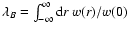The same magnetic power spectrum can have very different realizations, since all the phase information is lost in measuring the power spectrum (for an instructive visualisation of this see Maron & Goldreich 2001). Since the presented approach relies on the power spectrum only, it is not important if the magnetic fields are highly organised in structures like flux-ropes, or magnetic sheets, or if they are relatively featureless random-phase fields, as long as their power spectrum is the same.

The autocorrelation analysis is fully applicable in all such situations, as long as the fields are sampled with sufficient statistics. The fact that this analysis is insensitive to different realizations of the same power spectrum indicates that the method is not able to extract all the information which may be in the map. Additional information is stored in higher order correlation functions, and such can in principle be used to make statements about whether the fields are ordered or purely random (chaotic). The information on the magnetic field strength ($\vec{B}^2$, which is the value at origin of the autocorrelation function), and correlation length (an integral over the autocorrelation function) does only depend on the autocorrelation function and not on the higher order correlations.

The presented analysis relies on having a statistically isotropic sample of magnetic fields, whereas MHD turbulence seems to be locally inhomogeneous, which means that small scale fluctuations are anisotropic with respect to the local mean field. However, whenever the observing window is much larger than the correlation length of the local mean field the autocorrelation tensor should be isotropic due to averaging over an isotropic distribution of locally anisotropic subvolumes. This works if not a preferred direction is superposed by other physics, e.g. a galaxy cluster wide orientation of field lines along a preferred axis. However, even this case can in principle be treated by co-adding the RM signal from a sample of clusters, for which a random distribution of such hypothetical axes can be assumed. In any case, it is likely that magnetic anisotropy also manifests itself in the Faraday rotation maps, since the projection connecting magnetic field configurations and RM maps will conserve anisotropy in most cases, except alignments by chance of the direction of anisotropy and the line-of-sight. The presence of anisotropy can therefore be tested, which is discussed later in great detail.

Since there are cases where already an inspection by eye seems to reveal the existence of magnetic structures like flux ropes or magnetic sheets, we briefly discuss their appearance in the autocorrelation and the area filling statistics of RM maps. As already stated, the presence of such structures does not limit our analysis, as long as they are sufficiently sampled. Otherwise, one has to replace e.g. the isotropy assumption by a suitable generalisation. In many cases this will allow an analysis similar to the one proposed in this paper. We leave this for future work and applications where this might be required. A criteria to detect anisotropy statistically is given in this work.

1.4 Structure of the paper

In Sect. 2 the autocorrelation functions of magnetic fields and their RM maps are introduced, and their interrelation investigated. In Sect. 3 the same is done in Fourier space, which has not only technical advantages, but also provides insight into phenomena such as turbulence. Faraday map signatures of magnetic structures like flux-ropes are briefly discussed in Sect. 4. Possible pitfalls due to observational artefacts are investigated in Sect. 5. The conclusions in Sect. 6 summarise our main findings, and give references to the important results and formulae in detail.