A&A 401, 405-418 (2003)
DOI: 10.1051/0004-6361:20021853
3D continuum radiative transfer in complex dust
configurations around stellar objects
and active galactic nuclei
I. Computational methods and capabilities
J. Steinacker1 -
Th. Henning2 -
A. Bacmann3 -
D. Semenov1
1 - Astrophysical Institute and University Observatory
(AIU),
University of Jena,
Schillergässchen 2-3, 07745 Jena, Germany
2 -
Max Planck Institute for Astronomy, Königstuhl 17, 69117 Heidelberg, Germany
3 -
European Southern Observatory, Karl-Schwarzschild-Str. 2, 85748 Garching, Germany
Received 23 September 2002 / Accepted 9 December 2002
Abstract
We present the new grid-based code STEINRAY which has been developed
to solve the full 3D continuum radiative
transfer problem generally arising in the analysis of star-forming
regions, matter around evolved stars, starburst galaxies,
or tori around active galactic nuclei.
The program calculates the intensity emerging from these complicated
structures using a combination of step-size controlled ray-tracing and
adaptive multi-wavelength photon transport grids.
Along with a 2nd order finite differencing approach, the grids are
optimized to reduce the discretization error and provide
global error control.
The full wavelength-dependent problem is
solved without any flux approximation, and for arbitrary scattering
properties of the dust.
The program is designed to provide spatially resolved images, visibilities, and spectra
of complex dust distributions even without any symmetry for wavelengths ranging
from the UV to FIR and allows for
multiple internal and external sources.
In this paper, the algorithm is described and the capabilities of the
code are illustrated by the treatment of 1D and 3D test cases.
Analyzing the properties of typical cosmic dust, we
discuss the wavelength range for which
the time-consuming solution on adaptive grids can be omitted.
The temperature is calculated self-consistently using standard
accelerated  -iteration.
Key words: radiative transfer -
methods: numerical -
accretion, accretion disks -
ISM:
dust extinction
Nearly all information about astrophysical sources comes
from analyzing the radiation we receive from the objects.
Therefore, radiative transport
(thereafter RT) is one of the most fundamental processes considered in astrophysics
whenever radiation is altered on its way from the source to the telescope.
The alteration can range from small perturbations like the reddening
of stellar light due to interstellar extinction or the change of
polarization due to the Faraday effect, to almost complete shielding at short
wavelengths and thermal re-emission at infrared and sub-millimeter wavelengths in the
case of deeply-embedded star-forming regions, envelopes, and evolved stars,
or tori around
active galactic nuclei.
In view of the complex structure
of the matter around these objects revealing filamentary, disk- or
ring-like distributions, simple 1D approximations often fail
to describe the observed images and spectral energy distributions,
making multi-dimensional RT mandatory.
But even for symmetric dust distributions, asymmetric source distributions
or boundary conditions like, e.g., a single star near the dust cloud boundary
have to be treated
with 3D RT.
This will be
even more necessary in the near future, as the oncoming interferometers such as
VLTI, Keck, and ALMA will reach
resolutions revealing details at milli-arcsecond level, hence
resolving complicated 3D structures like planetary gaps (Bryden et al. 1999;
D'Angelo et al. 2002),
density waves (Pfalzner et al. 2000),
interaction streamers (Günther & Kley 2002),
and disk warps (Bouvier et al. 1999).
But it is not only for explaining complex observational
data that flexible three-dimensional
RT programs are required.
3D Smooth-Particle Hydrodynamical (SPH) and Magneto-Hydrodynamical (MHD)
simulations are now available and
produce time-dependent density and temperature distributions of dust and
gas
in star-forming regions, proto-planetary disks,
and in dust tori around AGNs.
Without a 3D RT code, it is impossible to predict at which wavelengths
or by which telescope these 3D features
can be detected. Moreover, only with a 3D RT program can the validity
of the approximate RT used in 3D SPH/MHD simulations be verified.
In line RT, the existing codes often use coarse approximations
for the spatial resolution and the scattering to be able to handle the
numerically intensive calculation of the level population (e.g. Folini
& Walder 1999;
Uitenbroek 2001; and
references therein).
For 3D continuum RT, different methods have been
applied to solve the complex transport equation, but only a few codes are
available.
The advantage of
Monte-Carlo methods is the easy treatment of complex
density distributions, complicated scattering functions, and
polarization.
Monte-Carlo methods require high numbers of photons to cover
re-emission in all directions and to treat optically thick regions, which can
be reduced using elaborated concepts like immediate reradiation.
The major drawback, however, is that there is no global error control
when using Monte-Carlo schemes.
They have been applied for 3D configurations in the papers of
Egan & Shipman (1995),
Wolf et al. (1999), Wolf & Henning (1999)
incorporating polarization,
and Gordon et al. (2001), Misselt et al. (2001)
considering also transient heating.
Integrating the RT equation along the considered line of sight by
using a
ray-tracer is a very flexible method for
treating complex density configurations.
It provides full error control, but requires the implicit re-calculation of
the step size and becomes very time-consuming when the optical depth
is high, so that approximations have to be used.
The first solution was published by Yorke (1986) solving the wavelength-dependent
problem in flux-limited approximation and without self-consistent temperature
iteration.
Well-established in hydrodynamical simulations,
solutions on fixed grids can also be performed in RT using a
finite difference or short characteristics discretization.
However, resolution of all relevant structures for all
wavelengths is very hard to achieve for most astrophysical applications.
Given that the intensity depends on
wavelength, three spatial and two directional coordinates,
a decent resolution of 100 points in each variable
already leads to solution vectors with 1012 components, which is not possible to store simultaneously even in
supercomputers nowadays.
Together with the complicated
integro-differential type of the RT equation which makes application
of common sparse matrix solvers impossible, a solution of the
3D RT can only be achieved by using sophisticated adaptive grids and
fast solution algorithms.
Two 3D continuum RT grid codes are available.
Stenholm et al. (1991) solved the transport equation
on a regular grid
using 1st order finite differencing
with low spatial resolution.
Folini et al. (2003) have developed a code to solve the
optically thick, stationary, wavelength decoupled, and unpolarized NLTE
radiative transfer problem for moving media of a given density.
This publication is the second in a series presenting the new
grid-based 3D RT code STEINRAY which incorporates the use
of multi-wavelength adaptive photon transport grids to provide
global error control of the solution.
The underlying grid generation mechanism was described in
Steinacker et al. (2002b).
In this paper, the full discretization and solution strategy is given
including the self-consistent temperature iteration, as well as simple
test cases to show the capabilities of the code.
In another paper, we compare the results for a standard accretion disk
in a 2D benchmark project with three other RT codes (Pascucci et al. 2003).
Further publications will deal with
applications to circumbinary disks, warped disks, gaps in disks,
pre-stellar cores, and
dust tori around AGNs.
In Sect. 2, the continuum RT equation is described and the solution
strategy is outlined.
The optical properties of typical cosmic dust are briefly reviewed in Sect. 3 and
limiting wavelengths are derived to decide when time-consuming calculations
on the adaptive multi-wavelengths photon transport grids have to be performed.
The solution of the transport equation in the case of substantial scattering
is described in Sect. 4. Section 5 describes the discretization of the
temperature distribution.
The code is tested in Sect. 6 for simple 1D cases and a complex 3D application.
We summarize our findings in Sect. 7.
We describe the radiation field by
the total specific intensity
 ,
where
,
where
 gives the location in space,
  is the direction of the radiation, and
 its wavelength.
Starting with the boundary values, we can calculate
the transport of the radiation through the considered
domain by solving the stationary 3D RT equation
its wavelength.
Starting with the boundary values, we can calculate
the transport of the radiation through the considered
domain by solving the stationary 3D RT equation
with the Planck function B, the dust temperature T, and the
phase function p. For simplicity, we will skip the index of the intensity which indicates that it is defined per
wavelength interval.
The extincting properties of enshrouding matter are described by
the line and continuum absorption and scattering of the radiation by
dust grains and gas species
 |
|
|
(2) |
In this paper, we focus on the solution of (1) for continuum
radiation,
and consider the absorption and scattering by dust
only, omitting the subscript "dust'' in the rest of the text for clarity.
We will restrict our consideration to the use of dust
particles with one size and a specific
chemical composition. Equation (1) can also be used for a size
or composition
distribution of dust grains, but then each of the different dust species
will have its own temperature.
The physical quantities describing the efficiency to absorb and scatter the
incident radiation by an ensemble of dust grains can be written as
 |
|
|
(3) |
where
 is the gas density and
 are the mass absorption and scattering coefficients of the dust ensemble,
respectively.
are the mass absorption and scattering coefficients of the dust ensemble,
respectively.
Two source terms of radiation are explicitely given in
Eq. (1), namely scattering into the line of
sight and re-radiation by the dust particles.
The scattering into the direction
is described by the probability
 that radiation is scattered from the direction
  into ,
with the solid angle
into ,
with the solid angle  .
The second source is the re-radiation of the dust particles
.
The second source is the re-radiation of the dust particles
 .
.
Intensity and dust temperature are not independent. The radiation field
determines the temperature and in turn, the dust re-emission contributes to
the radiation field.
This couples the partial integro-differential RT equation to the
local energy balance equation describing how a dust particle is heated
by the source radiation and the radiation of all other particles.
The balance
equation for the energy density in local thermal equilibrium
at point
is
 |
|
|
(4) |
The temperature is denoted by
 to distinguish it from
temperatures arising from other
possible heating sources like viscous heating, cosmic rays, or
gas-grain collisions.
to distinguish it from
temperatures arising from other
possible heating sources like viscous heating, cosmic rays, or
gas-grain collisions.
A simultaneous treatment of the 3D RT and hydrodynamical (HD)
equations in one code is currently beyond the capabilities
of nowadays computers. HD simulations commonly use
an approximate RT to calculate radiative heating, while in turn,
RT codes can use the derived densities and the heating sources
to calculate the radiation field at a given
time or in a stationary picture.
In view of the substantial computational effort to solve the
3D transport equation, it is mandatory to use any approximation
that is allowed by the physical conditions.
With vanishing scattering integral, (1) becomes a 1st order differential
equation which can be solved without problems using ray-tracing.
To make use of this approximation, and
since the operators in the integro-differential Eq. (1) are linear in  ,
we can (following e.g. Efstathiou & Rowan-Robinson 1990)
split the total specific intensity into an unprocessed passing source
component I* that includes also the thermal contribution from
the dust, and a processed component I of radiation that has encountered scattering
,
we can (following e.g. Efstathiou & Rowan-Robinson 1990)
split the total specific intensity into an unprocessed passing source
component I* that includes also the thermal contribution from
the dust, and a processed component I of radiation that has encountered scattering
 |
(5) |
Substituting the source term to be
this leads to three equations
with the known contributions
 |
|
|
(10) |
 |
|
|
(11) |
and the abbreviation
 .
.
 represents the source and thermal radiation that
is scattered at the point
into the direction .
The source and thermal contribution to the heating is described by
represents the source and thermal radiation that
is scattered at the point
into the direction .
The source and thermal contribution to the heating is described by
 .
.
As intended by the split (5), the first transfer Eq. (7) can be transformed to a path
integral and thus easily be calculated using the formal exponential
solution. For an empirical optical data set, the numerical solution
is conveniently
derived for all wavelengths e.g. using fifth-order Runge-Kutta with adaptive stepsize control
(Press et al. 1992) as ray-tracing routine. This provides error control for the solution,
and can be used for all optical depths from thin to thick regions.
Moreover, it allows to treat multiple external and internal sources
of radiation.
The second Eq. (8) still has an integro-differential
form and requires a separate, more sophisticated treatment.
The third Eq. (9) allows to update the temperature
from an intensity that has been calculated assuming a fixed temperature
using a standard accelerated -iteration (Ng 1974).
In order to decide where the scattering integral becomes negligible
and when the solution of the RT equation I* can be calculated
by solving (7) easily,
the optical properties of the dust grains have to be investigated.
For the sake of comparison, we concentrate on homogeneous spherical particles
of a uniform size (radius  m) consisting of amorphous carbon
(Preibisch et al. 1993; Rouleau & Martin 1991)
or astro-silicate (Draine & Lee 1984; Draine 1985).
Their optical properties are calculated
by the Mie theory for spheres (Mie 1908) using the modified code of
Barber & Hill (1990).
m) consisting of amorphous carbon
(Preibisch et al. 1993; Rouleau & Martin 1991)
or astro-silicate (Draine & Lee 1984; Draine 1985).
Their optical properties are calculated
by the Mie theory for spheres (Mie 1908) using the modified code of
Barber & Hill (1990).
More complicated dust models like mixtures of (in)homogeneous spherical
particles of various sizes and compositions can be treated by the code
without difficulty, but at expense of longer computational time.
To illustrate the typical behavior of the optical properties, we show in
Fig. 1
the ratio of the scattering and absorption efficiency factors
of dust particles consisting of amorphous carbon for different
sizes a as a function of wavelength.
![\begin{figure}
\par\includegraphics[width=12cm,clip]{ac1_sca_abs.ps}
\end{figure}](/articles/aa/full/2003/14/aa3097/Timg51.gif) |
Figure 1:
Ratio of scattering and absorption efficency factor as function of
the wavelength. The different curves correspond to different particle
sizes a. Two solid lines at the values 2 and -2 limit the
regions where scattering and absorption is considered to dominate, respectively. |
| Open with DEXTER |
The ratio roughly remains around 1 for wavelengths smaller than the
particle size and drops for larger wavelengths following a

 -powerlaw.
In order to give a conservative criterion for
neglecting scattering,
we define the limiting wavelength
-powerlaw.
In order to give a conservative criterion for
neglecting scattering,
we define the limiting wavelength
 to be the wavelength
where the ratio has dropped to 10-2. For larger wavelengths, we
can omit solving (8) and directly derive the total intensity from (7).
In Fig. 2,
to be the wavelength
where the ratio has dropped to 10-2. For larger wavelengths, we
can omit solving (8) and directly derive the total intensity from (7).
In Fig. 2,
![\begin{figure}
\par\includegraphics[width=8.8cm,clip]{wav_sca_abs.ps}
\end{figure}](/articles/aa/full/2003/14/aa3097/Timg55.gif) |
Figure 2:
Limiting wavelength for which scattering can be neglected, plotted
as a function of particle size a for amorphous carbon (dotted) and astro-silicate
(solid). In the parts above the lines, absorption is more than a factor
of 100 stronger than scattering. |
| Open with DEXTER |
the limiting wavelength is plotted against particle size a for
amorphous carbon (dotted line) and astro-silicate (solid line).
Roughly following an a1.12-powerlaw, the line indicates
that for optical wavelengths, all particles of astrophysical
relevance larger than  m scatter the radiation. In the near IR, particles
with
m scatter the radiation. In the near IR, particles
with  m require scattering calculations.
But even at higher wavelengths around
m require scattering calculations.
But even at higher wavelengths around  m, particles larger
than
m, particles larger
than  m will scatter the radiation substantially.
Depending on a given particle size a and wavelength ,
the program
switches from direct solution of the scattering
Eqs. (7)-(9) for
 to the easier ray-tracing solution of (7) for
 with the limiting wavelength
 .
.
If scattering is important, beside the scattering cross section,
the phase function
describing the probability of
the incoming radiation to be scattered from the direction
into
also has to be specified. This is important, as for isotropic scattering,
when
 ,
(1) can be simplified.
Integrating over the solid angle, the scattering integral
disappears and the equation becomes an ordinary differential equation
,
(1) can be simplified.
Integrating over the solid angle, the scattering integral
disappears and the equation becomes an ordinary differential equation
![\begin{displaymath}\vec n \nabla_{\vec x}
{\cal J}(\lambda,\vec x)
= \kappa^{\r...
...c x)\
\left[B(\lambda,\vec x)-{\cal J}(\lambda,\vec x)\right]
\end{displaymath}](/articles/aa/full/2003/14/aa3097/img64.gif) |
(12) |
for the total mean intensity
 |
(13) |
which is easy to solve.
We show in Fig. 3 the phase function in polar coordinates for
homogenous silicate spheres of size  m for different
wavelengths.
m for different
wavelengths.
![\begin{figure}
\par\includegraphics[width=8.8cm,clip]{bsil_p11.ps}
\end{figure}](/articles/aa/full/2003/14/aa3097/Timg67.gif) |
Figure 3:
Scattering phase function in polar coordinates for homogenous
spherical silicate particle of size m for different wavelengths.
 denotes the mean complex refractive index for all three
plotted wavelengths and
denotes the mean complex refractive index for all three
plotted wavelengths and
 is the size parameter.
In the optical wavelength range, the scattering is strongly peaked in
the forward direction. is the size parameter.
In the optical wavelength range, the scattering is strongly peaked in
the forward direction. |
| Open with DEXTER |
Radiation that is traveling parallel to the x-axis will be scattered by
the dust particle at the origin with a probability p into a direction
described by  .
Commonly, also the size parameter
.
Commonly, also the size parameter
 is used which we give in the picture, as well as the complex refractive
index
of the silicate.
Evidently, in the optical wavelength range, forward scattering dominates,
making the direct use of any approximation like isotropic scattering
impossible. But even for the limiting case of Rayleigh scattering
(
is used which we give in the picture, as well as the complex refractive
index
of the silicate.
Evidently, in the optical wavelength range, forward scattering dominates,
making the direct use of any approximation like isotropic scattering
impossible. But even for the limiting case of Rayleigh scattering
(
 ), for which the phase
function is most symmetric, the ratio of the probability of the radiation
to be scattered in forward and in perpendicular direction still equals 2,
as can be seen in Fig. 4 (dash-dotted line).
), for which the phase
function is most symmetric, the ratio of the probability of the radiation
to be scattered in forward and in perpendicular direction still equals 2,
as can be seen in Fig. 4 (dash-dotted line).
![\begin{figure}
\par\includegraphics[width=8cm,clip]{asil_p11.ps}
\end{figure}](/articles/aa/full/2003/14/aa3097/Timg72.gif) |
Figure 4:
Scattering phase function in polar coordinates for homogenous
spherical silicate particle of size
 m for different wavelengths.
denotes the mean complex refractive index for all three
plotted wavelengths and
is the size parameter.
In the optical wavelength range, the scattering is peaked in the forward direction,
but approaches the Rayleigh scattering limit where the ratio between forward
and perpendicular scattered intensities becomes 2, for longer wavelengths. m for different wavelengths.
denotes the mean complex refractive index for all three
plotted wavelengths and
is the size parameter.
In the optical wavelength range, the scattering is peaked in the forward direction,
but approaches the Rayleigh scattering limit where the ratio between forward
and perpendicular scattered intensities becomes 2, for longer wavelengths. |
| Open with DEXTER |
Here, we have also plotted the phase function
for a smaller particle
m for different wavelengths.
Anisotropic scattering can become very important.
If the dust grains are, e.g., of size  m,
in the optically thin case, there will be just a few scattering events
before the radiation escapes the object, and the scattered radiation
is strongly peaked in the forward direction.
Assuming isotropic scattering, the scattered radiation will be more
homogeneous and substantially different from the anisotropic case.
We just mention as one prominent example the atmosphere of an accretion
disk where the matter has low density
and just a few scattering
events occur before the radiation escapes the object.
In particular, interpreting images obtained for edge-on accretion disks
at short wavelengths is impossible without using the correct anisotropic
phase function.
In the program, we always use the correct anisotropic phase function.
m,
in the optically thin case, there will be just a few scattering events
before the radiation escapes the object, and the scattered radiation
is strongly peaked in the forward direction.
Assuming isotropic scattering, the scattered radiation will be more
homogeneous and substantially different from the anisotropic case.
We just mention as one prominent example the atmosphere of an accretion
disk where the matter has low density
and just a few scattering
events occur before the radiation escapes the object.
In particular, interpreting images obtained for edge-on accretion disks
at short wavelengths is impossible without using the correct anisotropic
phase function.
In the program, we always use the correct anisotropic phase function.
If more than one dust size is considered, the phase function may differ substantially between the different sizes. For efficient mixing of
the dust grains (assuming the same density distribution
for all sizes), a mean scattering function may be defined to handle
the transport of the scattered part of the radiation approximatively.
In the following, we describe how the integro-differential Eq. (8) is discretized and solved in the program.
For the direction coordinates ,
we choose spherical coordinates
 ,
while Cartesian coordinates x,y,z are best suited
for spatial coordinates in 3D RT problems with complex density distributions.
Hence, (8) turns into
,
while Cartesian coordinates x,y,z are best suited
for spatial coordinates in 3D RT problems with complex density distributions.
Hence, (8) turns into
It is likely that close to the source, the radiation field will be
peaked in a certain direction. To minimize discretization errors,
the direction grid should be refined around this .
But as this refinement strongly varies with the location, a coupled
location and direction grid would have to be used, which is numerically
prohibitive.
Hence, we choose a direction grid that is equally spaced on the unit sphere
with as many grid points as can be afforded numerically.
Steinacker et al. (1996) have calculated equally spaced
nodes for the cubature of the unit sphere and
corresponding weights derived by evaluating special Gegenbauer
polynomials. The grid points have been obtained using a
special Metropolis algorithm to maximize the distance between the nodes.
We denote the number of nodes with
 ,
and typical numbers we use range between 49 and
400 for a dust particle size of
,
and typical numbers we use range between 49 and
400 for a dust particle size of  m.
In view of the strongly peaked phase function for larger dust
particles, higher numbers might be necessary to resolve the peak
appropriately.
For the wavelength, we introduce a logarithmic grid
m.
In view of the strongly peaked phase function for larger dust
particles, higher numbers might be necessary to resolve the peak
appropriately.
For the wavelength, we introduce a logarithmic grid
 (in
(in  ,
f is an
index, while
,
f is an
index, while
 denotes
 to the power of f)
with
to the power of f)
with  grid points, and
use trapezoidal logarithmic integration in all occurring integrals.
grid points, and
use trapezoidal logarithmic integration in all occurring integrals.
For the spatial discretization, we use the adaptive optimized
multi-wavelength photon transport grids presented in Steinacker et al. (2002b).
These grids are obtained with a refinement grid generator
to minimize the 1st order discretization error and
guarantee global error control for the solution of the radiative
transfer problem on the grid. For each wavelength grid point, a spatial grid is
calculated, so that the number
 of grid points per grid
depends on the wavelength. The three Cartesian coordinates are
xfs,yfs,zfs,
respectively, used at wavelength grid point f where
of grid points per grid
depends on the wavelength. The three Cartesian coordinates are
xfs,yfs,zfs,
respectively, used at wavelength grid point f where
 .
The numbering of the grid points by s is caused by the refinement
procedure which generates the adaptive grids. They will be renumbered with
respect to the boundary
conditions and the considered direction.
.
The numbering of the grid points by s is caused by the refinement
procedure which generates the adaptive grids. They will be renumbered with
respect to the boundary
conditions and the considered direction.
The intensity is therefore discretized by a solution vector with
 components,
reaching values around 106 for typical astrophysical applications.
Each
vector component of the intensity can be written as
components,
reaching values around 106 for typical astrophysical applications.
Each
vector component of the intensity can be written as
 |
(15) |
The derivative
 in (8) has to be calculated on the spatial grid in order
to treat the transport of scattered radiation properly.
Steinacker et al. (2002a) have shown
that 1st order finite differencing schemes introduce numerical
diffusion into the solution of the RT equation, completely blurring
the features of the solution.
We choose
2nd order finite differencing to approximate the derivative,
as 3rd order finite
differencing schemes have been shown in that paper
to be too time-consuming for 3D RT.
in (8) has to be calculated on the spatial grid in order
to treat the transport of scattered radiation properly.
Steinacker et al. (2002a) have shown
that 1st order finite differencing schemes introduce numerical
diffusion into the solution of the RT equation, completely blurring
the features of the solution.
We choose
2nd order finite differencing to approximate the derivative,
as 3rd order finite
differencing schemes have been shown in that paper
to be too time-consuming for 3D RT.
The notation for a use of a 2nd order
finite differencing scheme on an adaptively
refined grid is shown in Fig. 5a.
![\begin{figure}
\par\includegraphics[angle=-90,width=12cm,clip]{fig1a.ps}
\end{figure}](/articles/aa/full/2003/14/aa3097/Timg90.gif) |
Figure 5:
Panel a) Sketch of a refined grid and the location of the seven
point 2nd order finite differencing stencil centered at point A. In the
upper part, the points are labeled according to their numbering with respect
to point A along the x, y, and z-direction, respectively.
Point B marks the center of a stencil moved downward with respect to A,
with
the point C indicating a stencil point which is not located on the grid.
Panel b) Refined grid and two cell deep shadow grid for a direction
that is indicated in the small coordinate system at the bottom. |
| Open with DEXTER |
To calculate the unknown intensity at a given point
 in the grid,
we use the known intensities at the two preceding grid points along the
Cartesian axes, with respect to the considered ray propagation direction
(we indicated this direction in the small coordinate system in the
lower right corner of Fig. 5b).
In this notation, e.g.
the point preceding
in the grid,
we use the known intensities at the two preceding grid points along the
Cartesian axes, with respect to the considered ray propagation direction
(we indicated this direction in the small coordinate system in the
lower right corner of Fig. 5b).
In this notation, e.g.
the point preceding  along the x-axis has
the x-coordinate x-1. The set of seven points defines a stencil
that is moved through the grid in the course of solving the transport
equation for the scattered radiation.
As shown in Fig. 5a,
this may lead to situations where for a point
there is no second
preceding grid point. In that case, 8-point interpolations are
performed for the preceding cube to obtain the intensity at C.
along the x-axis has
the x-coordinate x-1. The set of seven points defines a stencil
that is moved through the grid in the course of solving the transport
equation for the scattered radiation.
As shown in Fig. 5a,
this may lead to situations where for a point
there is no second
preceding grid point. In that case, 8-point interpolations are
performed for the preceding cube to obtain the intensity at C.
In 2nd order approximation, the derivatives with respect to the point
(xfs,yfs,zfs) and suppressing the s index
read as
with
If,gj,k,l=If,g(xfj,yfk,zfl).
To abbreviate, we define the constants
| Arf |
 |
 |
(19) |
| Brf |
|
 |
(20) |
| Crf |
|
 |
(21) |
| Drf |
|
![$\displaystyle - \left[
\Delta r^f_{-1} + \Delta r^f_{-2}
\right]^2$](/articles/aa/full/2003/14/aa3097/img99.gif) |
(22) |
| Erf |
|
![$\displaystyle \left(r^f\right)^2 \Delta r^f_{-2} - \left(r^f_{-1}\right)^2
\lef...
...ta r^f_{-1} + \Delta r^f_{-2}
\right]
+ \left(r^f_{-2}\right)^2 \Delta r^f_{-1}$](/articles/aa/full/2003/14/aa3097/img100.gif) |
(23) |
with
![$r\in [x,y,z]$](/articles/aa/full/2003/14/aa3097/img101.gif) .
.
Inserting (16)-(23) into the radiative
transfer Eq. (14), we obtain
The known factors can be abbreviated as
and solving the equation system with respect to
If,g0,0,0 yields
 |
|
|
(28) |
| Vf,g0,0,0 |
|
 |
(29) |
| Uf,g0,0,0 |
|
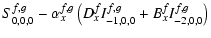 |
|
| |
|
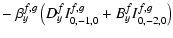 |
|
| |
|
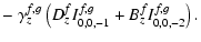 |
(30) |
With (28), we can calculate the intensity
of the scattered light at any grid point
when the intensities at the previous two grid points along the
three Cartesian axis are known. The density at the points
of the adaptive grid
is contained in
 and
Sf,g0,0,0.
and
Sf,g0,0,0.
The boundary values are defined on a shadow
grid that is not part of the adaptive photon grid. The boundary
intensities are determined by the interstellar radiation field
and nearby sources. As we use a 2nd order
differencing scheme, the shadow grid will be 2 cells deep.
Figure 5b shows such a shadow grid for a ray direction
with positive components
indicated by the arrow in the bottom right corner.
The cell size of the shadow grid will not influence the solution
and is chosen to be 1/10 of the computational domain.
Since intensities of radiation propagating in all directions are
calculated, the stencil will also be moved through the grid
in other directions than
the one following the orientation of the axis.
Equation (28) is also valid also for the down-winding case
(one of the components of direction vector
is negative)
if you re-order the grid points with respect to the direction vector
,
as can be shown by considering
rf0<rf-1<rf-2 with
![$r\epsilon[x,y,z]$](/articles/aa/full/2003/14/aa3097/img118.gif) .
.
A major numerical concern in 3D calculations is to reduce
the amount of calculations within the innermost loop of the
RT solver as much as possible.
In this loop, (7) and (8) are solved
by -iteration.
We therefore pre-calculate the positions
of all stencils for all directions. There are eight different direction
types to be considered ranging from all three Cartesian components
of
being positive to all being negative.
Beside that, the standard refinement used in generating the grids
guarantees that we can switch from a floating point storage of
the grid points to integer values as multiples of the smallest
occurring grid cell size. This reduces storage space of the grids and
increases the speed of the solution substantially.
Note that the solution scheme (28) has been derived for
a Cartesian grid, but equivalent schemes could be derived for
other coordinate systems.
![\begin{figure}
\par\includegraphics[width=16.8cm,clip]{grids.eps}
\end{figure}](/articles/aa/full/2003/14/aa3097/Timg119.gif) |
Figure 6:
Examples of temperature grids used by STEINRAY. Depending on the
density distribution, equidistant Cartesian a), spherical grids with
logarithmic radial points b), strongly overlapping nested Cartesian grids c),
cylindrical grids with logarithmic height griding d), and adaptive grids
with standard refinement e) are used. The number of grid points has been
reduced to keep the figure readable. |
| Open with DEXTER |
The overall solution strategy can be summarized as follows:
we specify a density distribution of the dust, its size
distribution, absorption and scattering properties, as well
as the scattering phase function. We define the location
and the spectrum of the radiation sources, and the boundary
conditions.
We specify the limiting wavelength for which we can neglect
scattering.
To start the computation, we analyze the density
distribution and determine minima, maxima and strong gradients.
Using the concept of penetration depths (see Steinacker et al. 2002b),
we construct adaptive photon transport grids for each wavelength.
For the temperature, we create another grid depending on the symmetry
of the density and source distribution. On this grid, we determine
a start temperature by illuminating each cell by the sources and
then each cell by each cell.
With this temperature T0, the unprocessed intensity I* is calculated
by solving (7). If scattering is important, also I is determined
by solving (8). In the latter case, we start with the scattered intensity
from the formerly treated wavelength and calculate the source term (6).
Then, the intensity is updated solving (8) with this source term
and this -iteration is continued until the intensity change
drops below a given value  (typically we choose
 ).
We use the standard technique proposed in Ng (1974)
to accelerate convergence by using former solutions.
).
We use the standard technique proposed in Ng (1974)
to accelerate convergence by using former solutions.
When
 has been calculated, we update the temperature using (9),
and continue this outer -iteration until the temperature has converged
to the self-consistent value.
During the iterations, we check the global energy to be conserved (and equal
to the start source energy).
has been calculated, we update the temperature using (9),
and continue this outer -iteration until the temperature has converged
to the self-consistent value.
During the iterations, we check the global energy to be conserved (and equal
to the start source energy).
It is possible to derive a priori guesses as to where the radiation
transport needs fine spatial grids to resolve the physics correctly
and hence to deduce the emerging radiation. Knowing the density
distribution and the optical properties of the dust particles,
the optical depth throughout a grid cell can be used
to derive a wavelength-dependent first order finite differencing criterion for the
grid generation (see Steinacker et al. 2002b). In most cases, this leads
to a refinement in the region around  .
For the temperature, this is hardly possible, as the temperature couples
to all wavelengths via (9) and hence, a clear definition of the
layer is not evident.
In regions where the radiation field is dominated by the source
contribution, the temperatures are expected to be high with high gradients.
Considering e.g. an accretion disk, strong temperature gradients
at the inner boundary and in the disk atmosphere are related to strong
density gradients.
For shielded regions, radiation is dominated by re-emitted long-wavelength
dust emission and the temperature gradients should be small.
.
For the temperature, this is hardly possible, as the temperature couples
to all wavelengths via (9) and hence, a clear definition of the
layer is not evident.
In regions where the radiation field is dominated by the source
contribution, the temperatures are expected to be high with high gradients.
Considering e.g. an accretion disk, strong temperature gradients
at the inner boundary and in the disk atmosphere are related to strong
density gradients.
For shielded regions, radiation is dominated by re-emitted long-wavelength
dust emission and the temperature gradients should be small.
Therefore, adaptively refining grids similar to the density grids
obtained in Steinacker et al. (2002b) could be used providing a global error control also for the temperature.
However, the use of two
different adaptive grids is very time-consuming. It has to be kept in
mind that both the ray-tracing solver and the scattering-integral
solver on the photon grids need the temperature at arbitrary points
within the computational domain, and this very often. An 8-point interpolation
is an acceptable effort, but with an adaptive grid, a tree-code search
algorithm is needed to find the corresponding grid cell, which is too
much of an effort especially for the scattering integral solver.
In view of the expected smooth behavior (compared to the radiation field)
of the temperature, simpler grids are used in STEINRAY with the
drawback of having no a-priori error control for the temperature. Some of them
are plotted in Fig. 6,
namely an equidistant Cartesian grid (a), a spherical grid with
radial points being logarithmically equidistant (b),
strongly overlapping nested Cartesian grids (c),
cylindrical grids with logarithmic height griding (d), and adaptive grids
with standard refinement (e) for cases where the same grid
for radiation and temperature can be used as the gradients within the object
are smooth.
The outer temperature iteration requires to start with a given initial
temperature distribution
 and then to improve
this distribution using (9)
to obtain the correct temperatures
and then to improve
this distribution using (9)
to obtain the correct temperatures  .
As this outer iteration requires to run the entire solution process
several times, it is essential to have quick
convergence and a good initial guess.
In the Appendix, we derive a scheme to calculate the initial
temperature distribution T0 for a given density distribution and optical
dust properties.
T0 is obtained neglecting scattering but considering both
stellar-cell and cell-cell illumination.
For deeply embedded
sources, the transformation of short-wavelength photons to infrared
radiation takes place in a thin dust layer, and as it matters little
for the overall temperature if the radiation is scattered there a
few times, T-T0 will be small and convergence fast.
If one deals with a configuration that has an extended atmosphere, namely
a region that can be seen from outside with an optical depth of the order
of 1 for wavelengths where scattering is important (like e.g. an accretion
disk), T0 and T will differ substantially in visible regions and thus
the images calculated from them will deviate too.
As we have pointed out in Sect. 3, forward scattering dominates the
scattering processes at wavelengths of strong scattering.
An improved T1 can be calculated using this effect:
in the source illumination of each cell, only the absorption
instead of the complete extinction is considered, arguing that the
radiation is not nearly lost but scattered forward in first approximation.
.
As this outer iteration requires to run the entire solution process
several times, it is essential to have quick
convergence and a good initial guess.
In the Appendix, we derive a scheme to calculate the initial
temperature distribution T0 for a given density distribution and optical
dust properties.
T0 is obtained neglecting scattering but considering both
stellar-cell and cell-cell illumination.
For deeply embedded
sources, the transformation of short-wavelength photons to infrared
radiation takes place in a thin dust layer, and as it matters little
for the overall temperature if the radiation is scattered there a
few times, T-T0 will be small and convergence fast.
If one deals with a configuration that has an extended atmosphere, namely
a region that can be seen from outside with an optical depth of the order
of 1 for wavelengths where scattering is important (like e.g. an accretion
disk), T0 and T will differ substantially in visible regions and thus
the images calculated from them will deviate too.
As we have pointed out in Sect. 3, forward scattering dominates the
scattering processes at wavelengths of strong scattering.
An improved T1 can be calculated using this effect:
in the source illumination of each cell, only the absorption
instead of the complete extinction is considered, arguing that the
radiation is not nearly lost but scattered forward in first approximation.
Testing RT codes is difficult as even in simple 1D cases,
for realistic density distributions, the RT equation already gets
too complicated to be solved analytically. Benchmark studies based on
well-defined RT problems can aid here to compare the results of different
codes. It may be pointed out here explicitly, though, that there may
be situations where the majority of codes fails, e.g. due to resolution
problems of standard algorithms. Only by incorporating error control is it
possible to infer reliability of the technique.
Hence, error control in STEINRAY will be one of the issues we will
discuss in the following.
For 1D continuum RT, a benchmark was published by Ivezic et al. (1997).
They compared results of three codes with similar algorithms for an
application in spherical geometry.
For 2D continuum RT, Pascucci et al. (2003) have defined a benchmark
based on simulations of a standard accretion disk around a solar-type
star. The project involved four separately developed codes, two based
on the Monte-Carlo technique and two based on grids, each with very
different implementation. STEINRAY has been tested in this collaboration
in good overall agreement with the other three codes.
There is no benchmark project for 3D continuum radiative transfer
yet. Hence, we present first results of the code two-folded:
we show simple test cases where the solution is either exactly or
approximately known, and a more complex 3D scenario to show the
capabilities. For applications to circumbinary disks, warped disks,
disks with planets, and AGN dust tori, as well for a 3D benchmark test
including images, we refer to the later papers
of this series.
In order to compare with an analytical solution, we start with the
most simple case possible, namely radiation passing through a
homogeneous dust medium with a constant density and no dust emission
radiation.
We follow the radiation up to a distance of 1000 AU from the source that is emitting
radiation just along the x-axis. For this so-called slab geometry, we assume
a constant dust number density of
1 m-3, spherical silicate dust particles of size
m, and a wavelength of  m so that scattering
can be neglected.
The optical depth
m so that scattering
can be neglected.
The optical depth
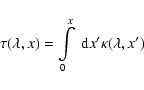 |
(31) |
along a ray (assumed to be parallel to the x-axis)
simplifies in this case to
 .
The solution of the continuum RT Eq. (1) then is
.
The solution of the continuum RT Eq. (1) then is
![${\cal I}(\lambda,x) = I_0 \exp{[-\tau(\lambda,x)]}$](/articles/aa/full/2003/14/aa3097/img129.gif) for all and vanishes for all directions except along the x-axis
for all and vanishes for all directions except along the x-axis
 .
Comparing the calculated intensity
.
Comparing the calculated intensity
 with the analytical
solution
with the analytical
solution
 ,
we can analyze the behavior of the used ray-tracer.
In Fig. 7,
we show the relative error
,
we can analyze the behavior of the used ray-tracer.
In Fig. 7,
we show the relative error
 in units of 10-3 as a function of x for a tracing with
constant steps (straight line) and with a 5th-order Runge Kutta
algorithm and adaptive step size control (noisy line). Both solutions have
errors below the given limit
in units of 10-3 as a function of x for a tracing with
constant steps (straight line) and with a 5th-order Runge Kutta
algorithm and adaptive step size control (noisy line). Both solutions have
errors below the given limit
 .
However, the adaptive step size solver
will automatically use the lowest number of points possible,
and works for any density distribution.
.
However, the adaptive step size solver
will automatically use the lowest number of points possible,
and works for any density distribution.
![\begin{figure}
\par\includegraphics[width=8.8cm,clip]{rterror.ps}
\end{figure}](/articles/aa/full/2003/14/aa3097/Timg135.gif) |
Figure 7:
Relative error of the intensity in a homogenous illuminated
cloud slab without continuum re-emission of the dust. The straight line
shows the error when using a constant stepsize tracer, the noisy
line gives the error of a 5th-order Runge Kutta-solver. |
| Open with DEXTER |
In spherical geometry, the intensity will spatially depend on the
radius only, and we can use the scaling argument by Ivezic et al. (1995)
to reduce the amount of free parameters in the 1D RT problem by
normalizing the occurring parameters.
We use the benchmark provided by
Ivezic et al. (1997) to test the code in spherical geometry. From their
models, we choose the scaled example of a central source with T*=2500 K,
a temperature at the inner boundary of T1=800 K, an outer
radius normalized to the inner boundary of Y=1000,
density power law index p=0 (constant density),
and optical depth at the
reference wavelength
 m to be
  .
For the sake of comparison, we also use isotropic scattering.
.
For the sake of comparison, we also use isotropic scattering.
We show the adaptive photon transport grid for the scattered radiation
at a wavelength of
 m in Fig. 8.
![\begin{figure}
\par\includegraphics[width=8.8cm,clip]{grid1dsph.ps}
\end{figure}](/articles/aa/full/2003/14/aa3097/Timg138.gif) |
Figure 8:
Adaptive photon transport grid for the scattered part of
the radiation passing through a dust envelope with spherically symmetric
density distribution, for the wavelength
m. |
| Open with DEXTER |
As the penetration
depth in this case is d=473 AU, the grid generator has just refined the
grid within a sphere of this radius to keep the optical depth across
one grid cell below the given error limit of
 .
The smallest cells are not plotted to keep the figure readable.
.
The smallest cells are not plotted to keep the figure readable.
The upper panel of
Fig. 9 shows the temperature we obtained (solid line)
along the z-axis as a function
of the normalized radius and the benchmark results (crosses).
![\begin{figure}
\par\includegraphics[width=8.8cm,clip]{spectemp.ps}
\end{figure}](/articles/aa/full/2003/14/aa3097/Timg141.gif) |
Figure 9:
Comparison with the 1D benchmark results of Ivezic et al. (1997)
for T1=800 K, Y=1000, p=0, ,
m,
and a resulting ratio  of incoming and re-radiated flux at the inner
boundary.
The upper panel shows the benchmark temperatures as a function of
normalized radius (crosses) and the result obtained with STEINRAY
(solid line).
In the lower panel, the dimensionless spectral shape
of incoming and re-radiated flux at the inner
boundary.
The upper panel shows the benchmark temperatures as a function of
normalized radius (crosses) and the result obtained with STEINRAY
(solid line).
In the lower panel, the dimensionless spectral shape
 d d
 is plotted in the same
notation.
is plotted in the same
notation. |
| Open with DEXTER |
We confirm
their findings and the agreement
was achieved after three outer -iterations.
The deviation of the temperatures at a given radius for all directions in the spherical
temperature grid was less than 1%.
In the lower panel of Fig. 9, the
normalized, distance- and luminosity-independent spectral energy distribution
d
is given
as a function of the wavelength. Again, there is good agreement between
benchmark result (crosses) and
STEINRAY simulation (solid line). The slight deviations might arise
from the different resolution of the grids.
Using the full symmetry of the problem, the 1D codes are able to spend all
the computer resources on resolving 1 dimension, while
the 3D code has to use a rather coarse grid of just
 wavelength grid points,
a direction grid of
wavelength grid points,
a direction grid of
 for the scattered radiation,
a spatial grid containing less than 105 cells per wavelength,
and temperature cell numbers fewer than 106 for the entire domain.
for the scattered radiation,
a spatial grid containing less than 105 cells per wavelength,
and temperature cell numbers fewer than 106 for the entire domain.
Tests with a 2D RT benchmark have been given in Pascucci et al. (2003)
comparing the results obtained with STEINRAY for a 2D standard accretion
disk with three other 2D and 3D RT codes. They show very good overall
agreement in both the spectrum and the temperature distribution.
We therefore proceed to full 3D RT. But here, no benchmark has been
defined sofar. And moreover, there is no benchmark yet that gives images
for multi-dimensional continuum RT. So, to show the capabilities of the
code, we just give here images of a complex test case and refer to further
applications and benchmark runs in forthcoming papers.
The example we choose is a spherically symmetric cloud core that contains
two young stars having formed at slightly different times, close to the
core center. We assume the stars to be massive (
 ),
with a luminosity of
),
with a luminosity of
 ,
and a surface temperature of T=20 000 K.
The emerging radiation is assumed to have already formed cavities free of dust, and all
remnants like disks that may have formed the stars are destroyed. We choose a slight time
shift in the evolution to have cavities with different sizes 1000 AU and
2000 AU, respectively, and at distances of 1500 and 2000 AU from the core center.
The stars are moved away from the cavity centers
towards the core center to distances of 1500AU and 1000 AU, respectively. This is to take into account the density gradient
within the core and its influence on the cavity formation.
The density within the core is assumed to
be a Gaussian of the form
,
and a surface temperature of T=20 000 K.
The emerging radiation is assumed to have already formed cavities free of dust, and all
remnants like disks that may have formed the stars are destroyed. We choose a slight time
shift in the evolution to have cavities with different sizes 1000 AU and
2000 AU, respectively, and at distances of 1500 and 2000 AU from the core center.
The stars are moved away from the cavity centers
towards the core center to distances of 1500AU and 1000 AU, respectively. This is to take into account the density gradient
within the core and its influence on the cavity formation.
The density within the core is assumed to
be a Gaussian of the form
![$\rho=\rho_0\ \exp[-r^2/r_0^2]$](/articles/aa/full/2003/14/aa3097/img146.gif) with
with  m-3and r0=2000 AU.
Figure 10 illustrates the density distribution in the z=0-plane.
![\begin{figure}
\par\includegraphics[width=8.8cm,clip]{density1.ps}
\end{figure}](/articles/aa/full/2003/14/aa3097/Timg148.gif) |
Figure 10:
Cut through the density distribution of the 3D test case at
z=0. The
two massive stars are located in cavities
that have formed within a dense core with a density maximum in-between
the two stars, their position is indicated by peaks. |
| Open with DEXTER |
The position
of the two stars is indicated by two peaks within the cavities. We consider this
scenario as a possible snapshot from the evolution of a dense core where two
stars have been formed and do not consider how stable this configuration will
be over longer time scales (a distortion of the core center due to gravitational
torque from the stars seems likely).
With this strongly asymmetric configuration, the stars displaced from the center
of the cavities of different size, and the inner core center between the stars,
clearly, 3D RT is needed to calculate the self-consistent temperature distribution
and to produce images for all wavelengths of interest. On the other side, the
configuration is still simple enough to allow for interpretation of the
obtained temperatures and images.
The calculated self-consistent temperature in the x-y-plane is shown in
Fig. 11.
In panel a, we show the temperature distribution
for a run where we placed just one star on the x-axis at x=-1500 AU.
The star heats the dust on its side of the core outside the cavity.
To heat up the opposite side of the core, its radiation has to pass the
inner core maximum and heating therefore is reduced. Radiation
passing through the small empty cavity, though, can reach the dust behind the
smaller cavity more easily than radiation not crossing the cavity.
Therefore, the dust directly behind the smaller cavity should be hotter than
dust that is heated by radiation not passing through the smaller cavity.
This effect can indeed be seen in panel a. Note that scattering blurs
this effect as for
 m, radiation is scattered out or into
the cavities.
In panel b, we give the temperature distribution when the other star
is added to the smaller cavity.
Due to the smaller extent of the small cavity, it is not able to heat the material
in the vicinity of the cavity to higher temperatures than the star in
the larger cavity, as the optical depth is higher.
In Fig. 12,
we show the images of the cavity configuration at wavelengths of
m, radiation is scattered out or into
the cavities.
In panel b, we give the temperature distribution when the other star
is added to the smaller cavity.
Due to the smaller extent of the small cavity, it is not able to heat the material
in the vicinity of the cavity to higher temperatures than the star in
the larger cavity, as the optical depth is higher.
In Fig. 12,
we show the images of the cavity configuration at wavelengths of
 m,
m,  m,
m,  m, and
  m,
respectively. The view is inclined by
m,
respectively. The view is inclined by  with respect to the
x-axis where both stars are located, and the smaller cavity is in the front.
with respect to the
x-axis where both stars are located, and the smaller cavity is in the front.
For
 m, the configuration is optically thin and the
dust emission at the surface of both
cavity shells accumulates so that they are clearly visible at all
viewing angles.
The re-emission function
m, the configuration is optically thin and the
dust emission at the surface of both
cavity shells accumulates so that they are clearly visible at all
viewing angles.
The re-emission function
![\begin{displaymath}R\equiv\kappa^{\rm abs}(\lambda,\vec x)\ B[\lambda,T(\vec x)]
\end{displaymath}](/articles/aa/full/2003/14/aa3097/img155.gif) |
(32) |
of the dust has its maximum for temperatures around
15 K, so emission should mainly be expected from the outer parts.
But due to the gradient of the Gaussian profile of the dense core,
radiation of the hotter dust at the surface of the cavities still dominates, which
radiates according to R with Planck emission in the Rayleigh-Jeans range.
The stars do not emit substantially at this wavelength.
![\begin{figure}
\par\includegraphics[width=16.6cm,clip]{cavtemp.eps}
\end{figure}](/articles/aa/full/2003/14/aa3097/Timg156.gif) |
Figure 11:
Temperature distribution of the cavity configuration in the
x-y-plane. a) Single star located on the x-axis at x=-1500 AU.
b) Two stars located on the x-axis at x=1000 AU and x=-1500 AU. |
| Open with DEXTER |
![\begin{figure}
\par\includegraphics[width=12.4cm,clip]{400x400_4pic.eps}
\end{figure}](/articles/aa/full/2003/14/aa3097/Timg157.gif) |
Figure 12:
Images of the cavity configuration at
m, m, m, and m,
respectively. The stars are located at x=1000 AU and -1500 AU on the
x-axis, the viewing angle is inclined by
so that the smaller
cavity is in the front. |
| Open with DEXTER |
At wavelength of
 m, the inner part of the core is
optically thick.
Part of the emission from the dust around the larger cavity is obscured
by the dense core.
The same is valid for the image at
m, the inner part of the core is
optically thick.
Part of the emission from the dust around the larger cavity is obscured
by the dense core.
The same is valid for the image at
 m. As the absorption
is stronger here, the smaller cavity is deeply embedded and emission is
only seen from parts where the density of the dense core drop due to the
Gaussian profile. In both pictures, emission from the star is too weak to
be seen.
m. As the absorption
is stronger here, the smaller cavity is deeply embedded and emission is
only seen from parts where the density of the dense core drop due to the
Gaussian profile. In both pictures, emission from the star is too weak to
be seen.
In the left upper panel of Fig. 12, the stars can be seen at
m (view along the y-axis, stars at x=1000 AU and -1500 AU,
total extend 10 000 AU). Still it is the dust close to the surface of the
cavity that is dominating the emission, but only the emission in the outer
parts can be seen as the extinction drops with the density.
The emission from the cavity surfaces is not entirely smooth, showing a
slight numerically caused ring pattern.
This is an effect of the finite grid size of 100 AU of the temperature
grid. Doubling the number of grid points in each direction (100 to 200)
would increase the size of the temperature array by a factor of 8 and the computational
time by a factor of 64. The use of an adaptive temperature grid reduces the
finite grid cell errors but increases the runtime as the interpolation
between the adaptive photon transport grid for the scattered radiation
and the temperature grid becomes more time-consuming.
The numerically by far most difficult part is to produce images in the
optical and UV. We have chosen
 m, as the scattering
is maximal in this wavelength range. With a deeply embedded pair of
stars like in our configuration, hardly any scattered light can be
expected to leave the core before being absorbed. As the images showed
just the reddened stars, we decided to lower the density by a factor
of 50 to make escape of scattered light possible.
We show two images at this wavelength in Fig. 13
with an inclination of the view by
m, as the scattering
is maximal in this wavelength range. With a deeply embedded pair of
stars like in our configuration, hardly any scattered light can be
expected to leave the core before being absorbed. As the images showed
just the reddened stars, we decided to lower the density by a factor
of 50 to make escape of scattered light possible.
We show two images at this wavelength in Fig. 13
with an inclination of the view by  with respect to the x-axis,
![\begin{figure}
\par\includegraphics[width=12.7cm,clip]{2picpaper.eps}
\end{figure}](/articles/aa/full/2003/14/aa3097/Timg162.gif) |
Figure 13:
Images of the cavity configuration at
m. The stars are located at x=1000 AU and -1500 AU on the
x-axis, the viewing angle is inclined by  so that the larger
cavity is in the front. The left image has been obtained using isotropic
scattering, the right image has been calculated with the correct
phase function.
so that the larger
cavity is in the front. The left image has been obtained using isotropic
scattering, the right image has been calculated with the correct
phase function. |
| Open with DEXTER |
and with the large cavity in the front.
The left image gives the intensity of scattered radiation calculated
under the assumption of isotropic scattering. Most emission comes from the
radiation scattered in the cavity. Its ring-like shape is an interplay
of the low density in the right part of the cavity reducing scattering
and the high density towards the center causing absorption.
There is also weak diffuse scattering in the entire core with
radial gradient following the density gradient.
The right image is calculated for the same viewing angle and wavelength,
but with a realistic scattering function as described in Sect. 3.
At
m, forward scattering dominates.
Therefore, only the front part of the surface of the larger cavity that is close to the star
and that has substantial density can scatter the radiation to the observer.
Additionally there is some diffuse scattered radiation coming from the front border
of the dense center of the core caused by the other star.
This comparison shows that a wrong approximation of the scattering
will alter the resulting images substantially.
Animations varying the viewing angle to support visualization of the
3D structure can be found under
http://www.astro. uni-jena.de/Users/stein/Ani/anin.htm.
Both ray-tracing and finite differencing on the transport grids
allow error control of the solution. Nevertheless, we point out that in contrast
to the intensity calculations, for the
temperature iteration, it is impossible to give an a priori error limit.
Here, we rely on usual a posteriori methods, namely to check the global
energy conservation when integrating the out-coming flux over a closed surface
around the source of energy. The main sources of numerical errors are the
interpolations of the temperatures for the ray-tracing and the transport grids.
As they have to be carried out often, a quadratic or higher polynomial interpolation is
too time-consuming. The same is valid for temperature grids with cell numbers
exceeding 106. For the simulations, global energy conservation within 5%
was used as convergence criterion for the outer -iteration.
In this paper, we presented the solution algorithm implemented
in the grid-based code STEINRAY, designed to
solve the 3D continuum radiative transfer problem for the intensity emerging
from objects in star-forming regions, evolved stars with envelopes,
starburst galaxies, and AGNs.
The method is a combination of step-size controlled ray-tracing and
solution on adaptive multi-wavelength photon transport grids, on which the
finite-differencing discretization error is minimized.
We briefly analyzed the optical properties of typical cosmic dust grains,
and discussed the wavelength range for which
the time-consuming solution on adaptive grids has to be used.
For the temperature, we have presented and discussed possible grids on which the
temperature distribution can be calculated self-consistently.
Aside from 2D benchmark comparisons presented elsewhere, we have tested the
code with simple 1D cases and illustrated the capabilities by treating a complex 3D test
case. The temperature is calculated self-consistently using standard accelerated
-iteration.
Acknowledgements
J. S. thanks F. Evans for valuable comments in the course of improving the
adaptive photon transport grids.
We thank D. Folini for an excellent referee report helping to
improve the paper at various points.
Computer time can be saved substantially when starting the solution
of the RT equation with a temperature that is already close to the
correct value. The temperature iteration in the RT solution
scheme will converge quickly
when an initial temperature is used that is derived for the case
that the high-energetic source radiation has been absorbed and
re-distributed by the dust particles already. Here, we derive a scheme to
calculate the initial temperature for a given dust configuration.
The main approximation is that the influence of scattering is
neglected for the heating process. In view of the strong forward
scattering in the wavelength regions where scattering plays a role,
this assumption is reasonable to derive an initial temperature
distribution.
We concentrate here on stellar illumination, but a corresponding
scheme can be derived for other radiation sources like evolved stars
or the central engine of an active galactic nucleus.
The power emitted by a star with the luminosity
 that is received by the dust particle k
of size a with the absorption efficiency
that is received by the dust particle k
of size a with the absorption efficiency
 at a distance rk through vacuum is (Evans 1994)
 |
(33) |
With R* and T* being the stellar radius and effective surface
temperature, respectively, the luminosity is
 and we get
 |
(34) |
Dividing the domain into  cell cubes of equal density and
temperature within the cube, with volume V,
the number of particles NK in a cell K can be obtained
from the number density
cell cubes of equal density and
temperature within the cube, with volume V,
the number of particles NK in a cell K can be obtained
from the number density  using
using
 |
(35) |
if a single-sized distribution of the dust is assumed.
Hence, the stellar power received at cell K writes as
 |
(36) |
where r*K is the distance between the star and cell K.
In the presence of extincting matter between star and dust,
the intensity along a ray
 from the star
to cell K is damped according to
from the star
to cell K is damped according to
 |
(37) |
with the unit vector
 pointing from the star to cell K, yielding
leaving the stellar power received at cell K to be
 |
(39) |
To define the temperature TK, we consider the power re-emitted by the
cell K in local thermal equilibrium
 |
(40) |
Hence, a starting temperature distribution T0 for the cells can be
obtained just from stellar illumination by setting
 for each cell. Inserting we find
 |
(41) |
In the next step, we consider that the cells illuminate each other.
The power that is received by cell L from cell K is
The total power received at cell L therefore is
 |
(43) |
The updated temperature TL1 yields from
 as
as
 |
| |
|
 |
(44) |
This formula applies also for the  iteration, where TL1 and
TL0 are exchanged by TLi+1 and TLi, respectively.
iteration, where TL1 and
TL0 are exchanged by TLi+1 and TLi, respectively.
Numerically,
 and
and
 are obtained from ray-tracing.
For large numbers of cells, ray-tracing should be truncated when the
intensity has dropped below a given limit characterizing a small
fraction of the thermal energy in the cell. In the optically thick
case, only cells located within a few mean free paths of the photons
will contribute to the cell-cell illumination.
are obtained from ray-tracing.
For large numbers of cells, ray-tracing should be truncated when the
intensity has dropped below a given limit characterizing a small
fraction of the thermal energy in the cell. In the optically thick
case, only cells located within a few mean free paths of the photons
will contribute to the cell-cell illumination.
We calculate
 |
(45) |
on a given wavelength grid  for
for
 and
use trapezoidal integration
and
use trapezoidal integration
![\begin{displaymath}\int F(x) {\rm d}x \approx \frac{1}{2}
\sum\limits_{f=2}^N
\left[ F(x_f)+F(x_{f-1}) \right] (x_f-x_{f-1}).
\end{displaymath}](/articles/aa/full/2003/14/aa3097/img196.gif) |
(46) |
The numerical scheme for calculating the temperature distribution
iteratively is
-
Barber, P. W., & Hill, S. C. 1990,
Light Scattering by Particles: Computational Methods
(World Scientific Publ. Co Pte Ltd)
In the text
-
Bouvier, J., Chelli, A., Allain, S., et al. 1999,
A&A, 349, 619
In the text
NASA ADS
-
Bryden, G., Chen, X., Lin, D. N. C., Nelson, R. P., & Papaloizou, C. B. 1999,
ApJ, 514, 344
In the text
NASA ADS
-
D'Angelo, G., Henning, Th., & Kley, W. 2002,
A&A, 2002, 385, 647
In the text
NASA ADS
-
Draine, B. T., & Lee, H. M. 1984,
ApJ, 285, 89
In the text
NASA ADS
-
Draine, B. T. 1985,
ApJS, 57, 587
In the text
NASA ADS
-
Efstathiou, A., & Rowan-Robinson, M. 1990,
MNRAS, 245, 275
In the text
NASA ADS
-
Egan, M. P., & Shipman, R. F. 1995,
AAS, 187, 100.05
In the text
-
Evans, A. 1994, The Dusty Universe (Wiley, New York)
In the text
-
Folini, D., & Walder, E. 1999,
IAUS, 193, 352
In the text
-
Folini, D., Walder, E., Psarros, M., & Desboeufs, A. 2003,
Stellar atmosphere modeling, PASP Conf. Ser., in press
In the text
-
Gordon, K. D., Misselt, K. A., Witt, A. N., & Clayton, G. C. 2001,
ApJ, 551, 269
In the text
NASA ADS
-
Günther, R., & Kley, W. 2002,
A&A, 387, 550
In the text
NASA ADS
-
Ivezic, Z., & Elitzur, M. 1995,
ApJ, 445, 415
In the text
NASA ADS
-
Ivezic, Z., Groenewegen, M. A. T., Men'shchikov, A., & Szczerba, R. 1997,
MNRAS, 291, 121
In the text
NASA ADS
-
Misselt, K. A., Gordon, K. D., Clayton, G. C., & Wolff, M. J. 2001,
ApJ, 551, 277
In the text
NASA ADS
-
Mie, G. 1908,
Ann. Phys., 25
In the text
-
Ng, K. 1974, J. Chem. Phys., 61, 2680
In the text
NASA ADS
-
Pascucci, I., Wolf, S., Steinacker, J., et al. 2003,
A&A, submitted
In the text
-
Pfalzner, S., Henning, Th., & Kley, W. 2000,
IAUS, 200, 193
In the text
-
Preibisch, Th., Ossenkopf, V., Yorke, H. W., & Henning, Th. 1993,
A&A, 279, 577
In the text
NASA ADS
-
Press, W. H., Teukolsky, S. A., Vetterling, W. T., & Flannery, B. P. 1992,
Numerical Recipes (Cambridge University Press, Cambridge)
In the text
-
Rouleau, F., & Martin, P. G. 1991,
ApJ, 377, 526
In the text
NASA ADS
-
Steinacker, J., Thamm, E., & Maier, U. 1996,
JQSRT, 56, 1, 97
In the text
-
Steinacker, J., Hackert, R., Steinacker, A., & Bacmann, A. 2002a,
JQSRT, 74, 183
In the text
NASA ADS
-
Steinacker, J., Bacmann, A., & Henning, Th. 2002b,
JQSRT, 75, 765
In the text
NASA ADS
-
Stenholm, L. G., Störzer, H., & Wehrse, R. 1991,
JQSRT, 45, 1, 47
In the text
NASA ADS
-
Uitenbroek, H. 2001,
ApJ, 557, 389
In the text
NASA ADS
-
Wolf, S., Henning, Th., & Stecklum, B. 1999,
A&A, 349, 839
In the text
NASA ADS
-
Wolf, S., & Henning, Th. 1999,
A&A, 341, 675
In the text
NASA ADS
-
Yorke, H. W. 1986,
in Astrophysical Radiation Hydrodynamics, ed. K.-H. Winkler,
& M. L. Norman (Reidel, Dordrecht), 141
In the text
Copyright ESO 2003
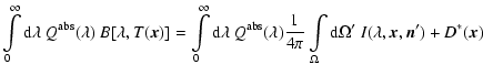
![\begin{figure}
\par\includegraphics[width=12cm,clip]{ac1_sca_abs.ps}
\end{figure}](/articles/aa/full/2003/14/aa3097/img51.gif)
![\begin{figure}
\par\includegraphics[width=8.8cm,clip]{wav_sca_abs.ps}
\end{figure}](/articles/aa/full/2003/14/aa3097/img55.gif)
![\begin{figure}
\par\includegraphics[width=8.8cm,clip]{bsil_p11.ps}
\end{figure}](/articles/aa/full/2003/14/aa3097/img67.gif)
![\begin{figure}
\par\includegraphics[width=8cm,clip]{asil_p11.ps}
\end{figure}](/articles/aa/full/2003/14/aa3097/img72.gif)
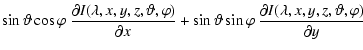
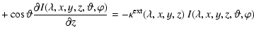
![\begin{figure}
\par\includegraphics[angle=-90,width=12cm,clip]{fig1a.ps}
\end{figure}](/articles/aa/full/2003/14/aa3097/img90.gif)
![$\displaystyle \left.\frac{\partial I}{\partial x}\right\vert _{x^f}\approx
\fra...
... x^f_{-2} + \Delta x^f_{-1}
\right]
+ \left(x^f_{-2}\right)^2 \Delta x^f_{-1}
}$](/articles/aa/full/2003/14/aa3097/img93.gif)
![$\displaystyle \left.\frac{\partial I}{\partial y}\right\vert _{y^f}\approx
\fra...
... y^f_{-2} + \Delta y^f_{-1}
\right]
+ \left(y^f_{-2}\right)^2 \Delta y^f_{-1}
}$](/articles/aa/full/2003/14/aa3097/img94.gif)
![$\displaystyle \left.\frac{\partial I}{\partial z}\right\vert _{z^f}\approx
\fra...
...z^f_{-2} + \Delta z^f_{-1}
\right]
+ \left(z^f_{-2}\right)^2 \Delta z^f_{-1}
},$](/articles/aa/full/2003/14/aa3097/img95.gif)
![$\displaystyle \frac{\sin\vartheta_g \cos\varphi_g}{E_x^f}
\left[
\left(C_x^f+A_...
...ight) I_{0,0,0}^{f,g}
+ D_x^f I_{-1,0,0}^{f,g}
+ B_x^f I_{-2,0,0}^{f,g}
\right]$](/articles/aa/full/2003/14/aa3097/img102.gif)
![$\displaystyle + \frac{\sin\vartheta_g \sin\varphi_g}{E_y^f}
\left[
\left(C_y^f+...
...ight) I_{0,0,0}^{f,g}
+ D_y^f I_{0,-1,0}^{f,g}
+ B_y^f I_{0,-2,0}^{f,g}
\right]$](/articles/aa/full/2003/14/aa3097/img103.gif)
![$\displaystyle + \frac{\cos\vartheta_g}{E_z^f}
\left[
\left(C_z^f+A_z^f\right) I_{0,0,0}^{f,g}
+ D_z^f I_{0,0,-1}^{f,g}
+ B_z^f I_{0,0,-2}^{f,g}
\right]=$](/articles/aa/full/2003/14/aa3097/img104.gif)


![\begin{figure}
\par\includegraphics[width=16.8cm,clip]{grids.eps}
\end{figure}](/articles/aa/full/2003/14/aa3097/img119.gif)
![\begin{figure}
\par\includegraphics[width=8.8cm,clip]{rterror.ps}
\end{figure}](/articles/aa/full/2003/14/aa3097/img135.gif)
![\begin{figure}
\par\includegraphics[width=8.8cm,clip]{grid1dsph.ps}
\end{figure}](/articles/aa/full/2003/14/aa3097/img138.gif)
![\begin{figure}
\par\includegraphics[width=8.8cm,clip]{spectemp.ps}
\end{figure}](/articles/aa/full/2003/14/aa3097/img141.gif)
![\begin{figure}
\par\includegraphics[width=8.8cm,clip]{density1.ps}
\end{figure}](/articles/aa/full/2003/14/aa3097/img148.gif)
![\begin{figure}
\par\includegraphics[width=16.6cm,clip]{cavtemp.eps}
\end{figure}](/articles/aa/full/2003/14/aa3097/img156.gif)
![\begin{figure}
\par\includegraphics[width=12.4cm,clip]{400x400_4pic.eps}
\end{figure}](/articles/aa/full/2003/14/aa3097/img157.gif)
![\begin{figure}
\par\includegraphics[width=12.7cm,clip]{2picpaper.eps}
\end{figure}](/articles/aa/full/2003/14/aa3097/img162.gif)
![$\displaystyle B_\lambda(T_*)*\exp\left[-\pi a^2\
\ Q_\lambda^{\rm ext}
\ \int\limits_{0}^{u_K} {\rm d} u'\ n(u') \right]$](/articles/aa/full/2003/14/aa3097/img176.gif)
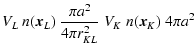
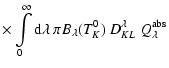
![$\displaystyle { \sum\limits_{f=2}^{N_\lambda}
\left[ B_{\lambda_f}(T_L^{i+1})\ ...
...1}}(T_L^{i+1})\ Q_{\lambda_{f-1}}^{\rm abs} \right]
(\lambda_f-\lambda_{f-1})=}$](/articles/aa/full/2003/14/aa3097/img197.gif)
![$\displaystyle \frac{1}{4}
\ \left(\frac{R_*}{r_{*L}}\right)^2
\sum\limits_{f=2}...
...L}^{i,\lambda_f} + W_{*L}^{i,\lambda_{f-1}} \right]
\ (\lambda_f-\lambda_{f-1})$](/articles/aa/full/2003/14/aa3097/img198.gif)
![$\displaystyle + \frac{1}{4}
\sum\limits_{K=1}^{Nc}
V_K\ n(\vec x_K)\
\frac{a^2}...
...}^{i,\lambda_f} + W_{KL}^{i,\lambda_{f-1}} \right]
\ (\lambda_f-\lambda_{f-1}).$](/articles/aa/full/2003/14/aa3097/img199.gif)