Because Vela X-1 is known to have a significant eccentricity, simply fitting
a sinusoidal radial velocity curve to the cross-correlation results as a
function of time would not be satisfactory, as an eccentric orbit will show
deviations from a pure sinusoid. Instead it may be shown that the
observed radial velocity is given by:
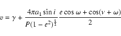 |
(10) |
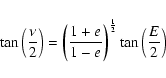 |
(11) |
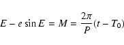 |
(12) |
The value of T0 was obtained from the value of ![]() ,
the epoch
of 90
,
the epoch
of 90![]() mean orbital longitude, derived by Bildsten et al. (1997)
from BATSE pulse timing data. They give
mean orbital longitude, derived by Bildsten et al. (1997)
from BATSE pulse timing data. They give
![]() ,
from which
,
from which
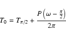 |
(13) |
Times, t, were assigned to each radial velocity measurement and
Eq. (12) was solved using a numerical grid to calculate the corresponding
eccentric anomaly. The true anomaly was then found using Eq. (11), and
Fig. 2 shows a plot of radial velocity against true anomaly, with the best
fit curve according to Eq. (10). The reduced chi-squared of the fit
is
![]() .
Scaling the error bars by a factor of 1.96 to
reduce
.
Scaling the error bars by a factor of 1.96 to
reduce
![]() to unity, gives the amplitude of the fitted curve
as
to unity, gives the amplitude of the fitted curve
as
![]() km s-1. However, we note
that, since the use of chi-squared assumes that the errors on all the points
are uncorrelated, the uncertainty here is likely to be a gross under-estimate.
This will hereafter be referred to as the "first fit''.
km s-1. However, we note
that, since the use of chi-squared assumes that the errors on all the points
are uncorrelated, the uncertainty here is likely to be a gross under-estimate.
This will hereafter be referred to as the "first fit''.
Figure 3 shows the residuals to the radial velocity curve in the first fit,
plotted against time. It is clear that there are trends apparent in these
residuals from night to night and a Fourier analysis shows that the dominant
signals are at periods of ![]() d and
d and
![]() d (Fig. 4).
The 9 d signal present in the power spectrum reflects the fact that fixing
the zero phase of the radial velocity curve, as implied by the X-ray data of
Bildsten et al. (1997) does not provide the best fit to the data. We suggest
this effect may be responsible for the "phase-locked'' deviations revealed
by Barziv et al. (2001) too. The 2.18 d modulation appears to be relatively
stable throughout our two orbits of observations, with an amplitude of around
5 km s-1, as shown in Fig. 3.
d (Fig. 4).
The 9 d signal present in the power spectrum reflects the fact that fixing
the zero phase of the radial velocity curve, as implied by the X-ray data of
Bildsten et al. (1997) does not provide the best fit to the data. We suggest
this effect may be responsible for the "phase-locked'' deviations revealed
by Barziv et al. (2001) too. The 2.18 d modulation appears to be relatively
stable throughout our two orbits of observations, with an amplitude of around
5 km s-1, as shown in Fig. 3.
![\begin{figure}
\par\includegraphics[angle=-90,width=8.8cm,clip]{H4013F3.ps}\end{figure}](/articles/aa/full/2003/13/aah4013/img82.gif) |
Figure 3: Residuals to the radial velocity curve fit in Fig. 2, plotted against time. (The first fit.) Overlaid is a best-fit sinusoid with a period of 2.18 d. |
![\begin{figure}
\par\includegraphics[angle=-90,width=8.8cm,clip]{H4013F4.ps}\end{figure}](/articles/aa/full/2003/13/aah4013/img85.gif) |
Figure 4:
Power spectra of the residuals to the radial velocity curve fits.
The solid curve is the power spectrum of the data in Fig. 3 (the residuals
after the first fit) and the dotted curve (offset in the -ve direction
by one unit for clarity) is the power spectrum of the data
in Fig. 6 (the residuals after the second fit). The highest peaks in
the power spectrum of the residuals after the first fit correspond to
frequencies of
|
In order to take account of the correlated residuals from the first fit,
another fit to the radial velocity data was performed this time with four free
parameters: the ![]() velocity and the
velocity and the ![]() value as before, plus the
amplitude and phase of a sinusoid with a period of 2.18 d. The
value as before, plus the
amplitude and phase of a sinusoid with a period of 2.18 d. The ![]() part of the fit is sinusoidal as a function of true anomaly, whilst the 2.18 d
part of the fit is sinusoidal purely as a function of time. The radial velocity
fit according to this prescription, referred to as the second fit, is shown in
Fig. 5 and has a reduced chi-squared of 2.40. The improvement over the first
fit is therefore clearly apparent. Scaling the error bars by a factor of 1.55
to reduce
part of the fit is sinusoidal as a function of true anomaly, whilst the 2.18 d
part of the fit is sinusoidal purely as a function of time. The radial velocity
fit according to this prescription, referred to as the second fit, is shown in
Fig. 5 and has a reduced chi-squared of 2.40. The improvement over the first
fit is therefore clearly apparent. Scaling the error bars by a factor of 1.55
to reduce
![]() to unity, gives the amplitude of the fitted curve
as
to unity, gives the amplitude of the fitted curve
as
![]() km s-1 and the amplitude of the 2.18 d
modulation as
km s-1 and the amplitude of the 2.18 d
modulation as
![]() km s-1. As with the first fit, we note
that the uncertainties here are also likely to be under-estimates. The
remaining residuals on the second fit are shown in Fig. 6, and their power
spectrum is indicated by the dotted line in Fig. 4. It can be seen that some
of the correlated structure in the residuals has been removed by this
procedure, although the peak corresponding to a period of
km s-1. As with the first fit, we note
that the uncertainties here are also likely to be under-estimates. The
remaining residuals on the second fit are shown in Fig. 6, and their power
spectrum is indicated by the dotted line in Fig. 4. It can be seen that some
of the correlated structure in the residuals has been removed by this
procedure, although the peak corresponding to a period of ![]() 9 d is
still present indicating once again that the zero phase according to the X-ray
observations does not provide the best description.
9 d is
still present indicating once again that the zero phase according to the X-ray
observations does not provide the best description.
![\begin{figure}
\par\includegraphics[angle=-90,width=8.8cm,clip]{H4013F6.ps}\end{figure}](/articles/aa/full/2003/13/aah4013/img90.gif) |
Figure 6: Residuals to the radial velocity curve fit in Fig. 5, plotted against time. (The second fit.) |
To test whether the deviations from the radial velocity curve
displayed by each group of data points are correlated, we subtracted the
effect of the 2.18 d period according to the parameters found for it
in the second fit, and rebinned the resulting radial velocities into nine
phase bins (each ![]() 1 day). The radial velocity fit to these phase-binned
means is shown in Fig. 7 and has a reduced chi-squared of 28.3. The errors
on the mean data points are calculated as the standard error on the mean
from the individual data points that are averaged in each case. The fact that
the reduced chi-squared is significantly greater than unity suggests that
the deviations are indeed correlated. Scaling the error bars here by a factor
of 5.3 to reduce
1 day). The radial velocity fit to these phase-binned
means is shown in Fig. 7 and has a reduced chi-squared of 28.3. The errors
on the mean data points are calculated as the standard error on the mean
from the individual data points that are averaged in each case. The fact that
the reduced chi-squared is significantly greater than unity suggests that
the deviations are indeed correlated. Scaling the error bars here by a factor
of 5.3 to reduce
![]() to unity, gives the amplitude of the fitted
curve as
to unity, gives the amplitude of the fitted
curve as
![]() km s-1.
km s-1.
Figure 7 clearly shows that a better fit would be obtained if the zero phase of
the radial velocity is allowed as a free parameter. This reflects the fact
that a ![]() 9 d period is present in the power spectra of the residuals after
both the first and second fits (Fig. 4). Allowing the zero phase to vary
results in the second fit to the phase binned data shown by the dashed
line in Fig. 7. This time the reduced chi-squared is 6.0.
Scaling the error bars here by a factor of 2.44 to reduce
9 d period is present in the power spectra of the residuals after
both the first and second fits (Fig. 4). Allowing the zero phase to vary
results in the second fit to the phase binned data shown by the dashed
line in Fig. 7. This time the reduced chi-squared is 6.0.
Scaling the error bars here by a factor of 2.44 to reduce
![]() to
unity, gives the amplitude of the fitted curve as
to
unity, gives the amplitude of the fitted curve as
![]() km s-1. The shift of the minimum radial velocity with respect to
that in the first fit to the pase binned means is a true anomaly of
km s-1. The shift of the minimum radial velocity with respect to
that in the first fit to the pase binned means is a true anomaly of
![]() ,
corresponding to about 7 hours. We note that this shift in zero phase is significantly greater than the
uncertainty implied by extrapolating the X-ray ephemeris of Bildsten et al.
(1997) to the epoch of our observations which is only
,
corresponding to about 7 hours. We note that this shift in zero phase is significantly greater than the
uncertainty implied by extrapolating the X-ray ephemeris of Bildsten et al.
(1997) to the epoch of our observations which is only ![]() 0.0006 of a cycle.
We conclude that the orbital phase locked deviations remaining in
the radial velocities after the first fit to means can therefore
mostly be accounted for by a simple phase shift in the radial velocity curve.
0.0006 of a cycle.
We conclude that the orbital phase locked deviations remaining in
the radial velocities after the first fit to means can therefore
mostly be accounted for by a simple phase shift in the radial velocity curve.
Copyright ESO 2003
![\begin{figure}
\par\includegraphics[angle=-90,width=8.8cm,clip]{H4013F5.ps}\end{figure}](/articles/aa/full/2003/13/aah4013/img89.gif)
![\begin{figure}
\par\includegraphics[angle=-90,width=8.8cm,clip]{H4013F7.ps}\end{figure}](/articles/aa/full/2003/13/aah4013/img92.gif)