Both the spectroscopic as well as the photometric time-series were analysed with the program package TRIPP. It enables the calculation of periodograms, confidence levels and fits with multiple sine functions (see Dreizler et al. 2002 for more details).
We were able to derive accurate radial velocity curves for the Balmer lines
![]() and
and
![]() (see Fig. 2). The
frequency resolution for this run is calculated to be 51
(see Fig. 2). The
frequency resolution for this run is calculated to be 51
![]() Hz. Trailing mode observations require stable weather conditions so that
the intensity of the star's signal is almost constant during one exposure. Thus
bad seeing and transparency changes due to the passage of small clouds influence
the quality of the data rather strongly. Because of these disturbances the
quality of the radial velocity curves varies with time. The radial velocity
curves of the other Balmer lines and the He lines turned out to be too noisy for
a quantitative analysis and are not further discussed. Better conditions should
allow a more extensive study of radial velocity changes in this star.
Hz. Trailing mode observations require stable weather conditions so that
the intensity of the star's signal is almost constant during one exposure. Thus
bad seeing and transparency changes due to the passage of small clouds influence
the quality of the data rather strongly. Because of these disturbances the
quality of the radial velocity curves varies with time. The radial velocity
curves of the other Balmer lines and the He lines turned out to be too noisy for
a quantitative analysis and are not further discussed. Better conditions should
allow a more extensive study of radial velocity changes in this star.
The Lomb-Scargle periodograms calculated from the radial velocity curves (see
Fig. 3) show peaks clearly surpassing the 3![]() confidence
level. Applying a prewhitening procedure to the data three frequencies and their
amplitudes (see Table 1) were found for both Balmer lines
investigated. Other peaks that seem
to lie above the 3
confidence
level. Applying a prewhitening procedure to the data three frequencies and their
amplitudes (see Table 1) were found for both Balmer lines
investigated. Other peaks that seem
to lie above the 3![]() level could not be extracted by our procedure. The
dominant frequency at 2.076 mHz has the largest velocity amplitude with 12.7 km s-1 for
level could not be extracted by our procedure. The
dominant frequency at 2.076 mHz has the largest velocity amplitude with 12.7 km s-1 for
![]() and 14.3 km s-1 for
and 14.3 km s-1 for
![]() .
The
amplitudes of the other two frequencies are lower than the strongest one with
values ranging from 6 to 8 km s-1. We determined the amplitude accuracy
.
The
amplitudes of the other two frequencies are lower than the strongest one with
values ranging from 6 to 8 km s-1. We determined the amplitude accuracy
![]() by calculating the
median value of the white noise in the frequency range 3-7 mHz where almost
no power arises in the frequency spectrum. According to this, we found
by calculating the
median value of the white noise in the frequency range 3-7 mHz where almost
no power arises in the frequency spectrum. According to this, we found
![]() = 1.5 km s-1 for
= 1.5 km s-1 for
![]() and
and ![]() = 1.0 km s-1 for
= 1.0 km s-1 for
![]() .
.
![\begin{figure}
\par\includegraphics[width=7.5cm,clip]{3408.f2.eps}\par\vspace*{4mm}
\includegraphics[width=7.5cm,clip]{3408.f3.eps}\end{figure}](/articles/aa/full/2003/13/aa3408/img27.gif) |
Figure 2:
Radial velocity curve for
|
BUSCA is a unique instrument which enables the measurement in four different wave bands simultaneously. As a result we obtained four light curves.
Figure 4 shows the Lomb-Scargle periodograms of all BUSCA bands. They
are quite similar to the periodograms derived from the radial velocity curves
(Fig. 3). This data set spans over three nights so that daily aliases
are clearly visible and the frequency resolution is much better at
![]() Hz (compared to 51
Hz (compared to 51 ![]() Hz for the spectroscopy). Again we applied
the prewhitening technique in order to remove all significant peaks from the
periodogram and to obtain the amplitudes for each frequency. As
before, the horizontal line in the diagrams represents the 3
Hz for the spectroscopy). Again we applied
the prewhitening technique in order to remove all significant peaks from the
periodogram and to obtain the amplitudes for each frequency. As
before, the horizontal line in the diagrams represents the 3![]() confidence level above which we assume the detected frequencies to be real. In
all four wave bands five peaks with the same frequencies can be identified
(see Tables 2 and 3). The dominant frequency is again found
at 2.076 mHz and therefore confirms the results from spectroscopy. Furthermore,
additional frequencies were found in the region around 2.74-2.78 mHz but
these peaks are closely spaced so that a corresponding identification in all
BUSCA bands due to the medium frequency resolution was not possible. Peaks
that fall below the 3
confidence level above which we assume the detected frequencies to be real. In
all four wave bands five peaks with the same frequencies can be identified
(see Tables 2 and 3). The dominant frequency is again found
at 2.076 mHz and therefore confirms the results from spectroscopy. Furthermore,
additional frequencies were found in the region around 2.74-2.78 mHz but
these peaks are closely spaced so that a corresponding identification in all
BUSCA bands due to the medium frequency resolution was not possible. Peaks
that fall below the 3![]() confidence level were not removed from the
periodograms.
confidence level were not removed from the
periodograms.
The amplitudes of the brightness variations are measured in fractional
intensity. The light curves are normalized to the fraction of intensity
![]() and the amplitudes were then converted to mmag.
This unit will be used throughout the whole paper.
The accuracy of these amplitudes are
calculated in the same way as we did it for the radial velocity amplitudes. Here
we used the median level of the white noise in the range 3-5 mHz. The
accuracies for the BUSCA wavebands are 1.52 mmag for "
and the amplitudes were then converted to mmag.
This unit will be used throughout the whole paper.
The accuracy of these amplitudes are
calculated in the same way as we did it for the radial velocity amplitudes. Here
we used the median level of the white noise in the range 3-5 mHz. The
accuracies for the BUSCA wavebands are 1.52 mmag for "
![]() '', 1.53 mmag for "
'', 1.53 mmag for "
![]() '', 1.12 mmag for
"
'', 1.12 mmag for
"
![]() '' and 1.37 mmag for "
'' and 1.37 mmag for "
![]() '', respectively.
'', respectively.
Figure 5 shows the semi amplitudes of four selected frequencies as a
function of effective wavelength of the bands. In Fig. 6
we display the relative change of the semi amplitude of each waveband. The
deviation with respect to the mean is largest for the "
![]() '' band.
The other channels, considered separately, behave rather similar showing much
smaller deviations from the mean brightness. This is explained
through the fact that the "
'' band.
The other channels, considered separately, behave rather similar showing much
smaller deviations from the mean brightness. This is explained
through the fact that the "
![]() '' band lies blueward to
the Balmer jump and the other redward of it. The opacity changes a lot across
this wavelength range and thus the stellar flux originates from different
atmospheric depths.
'' band lies blueward to
the Balmer jump and the other redward of it. The opacity changes a lot across
this wavelength range and thus the stellar flux originates from different
atmospheric depths.
Furthermore, we used the phases which are delivered by the sine fit
procedure (see Tables 2 and 3) in order to test whether there
is any wavelength dependency. The phase values are normalized to unity.
Figure 7
shows the deviations of the phases with respect to the mean value of all four
wavebands for the four selected frequencies of Fig. 5. The error bars
are calculated from
| (1) |
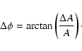 |
(2) |
![\begin{figure}
\par\includegraphics[width=8.8cm,clip]{3408.f10.eps}\end{figure}](/articles/aa/full/2003/13/aa3408/img35.gif) |
Figure 5:
Semi amplitudes of four frequencies as a function of effective
wavelength. The error bars are 1 |
Copyright ESO 2003
![\begin{figure}
\par\includegraphics[width=7.5cm,clip]{3408.f4.eps}\par\vspace*{4mm}
\includegraphics[width=7.5cm,clip]{3408.f5.eps}\end{figure}](/articles/aa/full/2003/13/aa3408/img29.gif)
![\begin{figure}
\par\includegraphics[width=7.3cm,clip]{3408.f6.eps}\par\vspace*{2...
...ps}\par\vspace*{2mm}
\includegraphics[width=7.3cm,clip]{3408.f9.eps}\end{figure}](/articles/aa/full/2003/13/aa3408/img30.gif)