A&A 400, 1129-1144 (2003)
DOI: 10.1051/0004-6361:20030065
H. Beust
Laboratoire d'Astrophysique de Grenoble, Université J. Fourier, BP 53, 38041 Grenoble Cedex 9, France
Received 30 September 2002 / Accepted 19 December 2002
Abstract
Symplectic integration has been used successfully for many
years now for the study of dynamics in planetary systems. This technique
takes advantage of the fact that in a planetary system, the mass of
the central body is much larger than all the other ones; it fails if
all massive bodies have comparable masses, such as in multiple stellar
systems. A new symplectic integrator is presented that permits the
study of the dynamics of hierarchical stellar systems of any size and
shape, provided that the hierarchical structure of the system is preserved
along the integration. Various application tests of this new integrator
are given, such as the gap formation in circumbinary disks, the Kozai
resonance in triple systems, the truncated circumbinary disk in the
quadruple system GG Tauri, and the dynamics of the sextuple system Castor.
Key words: methods: N-body simulations - methods: numerical - celestial mechanics - stars: binaries: general - stars: circumstellar matter
Symplectic integrators have become very popular in the last decade in planetary dynamics problems, as they present two major advantages with respect to other n-body integrators: First, they exhibit no long-term accumulation of energy error, and second they provide a gain of at least one order of magnitude in computation speed, for equivalent accuracy, because they allow one to adopt a much larger time-step than other integrators for the same result, leading to a much more rapid integration. The most popular symplectic integrator is the second-order MVS (Mixed Variable Symplectic) one, first described by Wisdom & Holman (1991) and implemented by Levison & Duncan (1994) in their SWIFT_MVS integration package.
The general assumption for efficient symplectic integrators is that the the motion of each body is separated into a dominant Keplerian part, solved to machine precision with an appropriate algorithm, and a perturbation that is solved numerically. In planetary dynamics, the dominant Keplerian part is due to the central star, and the perturbations to the planets. The MVS integrator is based on this assumption. However, the integration is no longer valid whenever the perturbation becomes larger than, or even of comparable order to the dominant Keplerian part. In planetary dynamics, this occurs when some of the bodies get close to each other, i.e., in the so-called case of close encounters. A large effort was done in the past years to make symplectic integrators handle close encounters (Levison & Duncan 1994; Chambers 1999; Duncan et al. 1998): The basic idea is to reduce the integration time-step during close encounters, but this necessarily no longer preserves the symplectic character of the integration, although from a statistical point of view, the results are still valid (Levison & Duncan 1994). Chambers (1999), in his MERCURY integrator, incorporates the close encounter perturbation into the Keplerian term during close encounters, but with the consequence of a significant decrease of the integration speed. Finally, Duncan et al. (1998), in their SyMBA integrator, use a multiple time-step technique that handles close encounters while remaining symplectic. However, it fails in integrating close encounters with the central star. A variant to this method is presented in Levison & Duncan (2000) that overcomes this difficulty but is more CPU-time consuming.
In planetary dynamics, the motion of the bodies is nearly Keplerian far from close encounters because the mass of the central star largely overcomes that of the other bodies. This is no longer valid in multiple stellar systems, where several massive centers can be present. Multiple stellar systems can be classified into two sets: Trapezian and Hierarchical systems. In trapezian systems, all relative distances between the bodies are more or less comparable. These systems are usually unstable on time-scales of a few Myrs or less, and it is very difficult in general to identify a dominant Keplerian part in the relative motion of their components. Hierarchical systems are conversely characterized by nested orbits of very different sizes, and are usually more stable. In that case, the motion of the bodies remains nearly Keplerian thanks to the very different size of the nested orbits, although all massive bodies may have comparable masses.
However, unless in specific cases, the MVS technique cannot be used
directly to compute the
dynamics of hierarchical multiple stellar system, as it needs to hold
one of the bodies as the "Sun'', and the other ones as the perturbing
"planets''. An interesting new technique dedicated to the study of
planets in binary systems was recently presented by Chambers et al. (2002),
with application to the ![]() Centauri system (Quintana et al. 2002). This
integrator is however limited to binary systems only. The
purpose of this paper is to present a new MVS-like integrator
dedicated to the integration of the dynamics of hierarchical systems
of any size and structure, provided the hierarchy is preserved. We
give this new method the name HJS (Hierarchical Jacobi Symplectic). In
Sect. 2, we briefly review the theory of symplectic integrators and
the MVS method, and develop the theory for the HJS method. Various
integration tests of growing complexity are given in Sect. 3.
Our conclusions are presented in Sect. 4.
Centauri system (Quintana et al. 2002). This
integrator is however limited to binary systems only. The
purpose of this paper is to present a new MVS-like integrator
dedicated to the integration of the dynamics of hierarchical systems
of any size and structure, provided the hierarchy is preserved. We
give this new method the name HJS (Hierarchical Jacobi Symplectic). In
Sect. 2, we briefly review the theory of symplectic integrators and
the MVS method, and develop the theory for the HJS method. Various
integration tests of growing complexity are given in Sect. 3.
Our conclusions are presented in Sect. 4.
An integration of any Hamiltonian system is symplectic when it exactly preserves the generalized areas in phase-space. This is in particular the case if the integration exactly solves (within computer round-off errors) a Hamiltonian. Symplectic integrators do not actually strictly solve the real Hamiltonian of the problem, but do it for a surrogate Hamiltonian assumed to be close to the real one. Once this is achieved it can be shown that there is no long-term drift of the energy. This is not the case for more classical methods (Runge-Kutta, Burlish & Stoer...) used in celestial mechanics, that are far from being symplectic.
The theory of symplectic integration is based on the Hamilton equations of
motion that apply to any n-body problem. Its background is for example
described in Saha & Tremaine (1992) and Chambers (1999).
The key idea of symplectic integration is to split the Hamiltonian H
the problem into pieces, say
| H=HA+HB, | (1) |
A second order integrator can be achieved if we combine now three sub-steps:
Additional accuracy is reached in symplectic integration if we have now
in addition
![]() ,
i.e.,
,
i.e.,
![]() with
with
![]() .
In that case we have
.
In that case we have
 |
(2) |
Let us consider
a general n-body gravitational system, with bodies labeled
from 1 to n, masses
![]() ,
positions
,
positions
![]() and impulsions
and impulsions
![]() in the barycentric
referential frame. Then the Hamiltonian of the system reads
in the barycentric
referential frame. Then the Hamiltonian of the system reads
| |
= | (4) | |
| = | (5) |
 |
(7) |
In Eq. (6), Wisdom & Holman (1991)
particularize the role of the first body #1, which appears
natural in the case of a planetary system (body #1 is the "Sun'').
H appears not to depend on the first Jacobi coordinate
![]() ,
showing as expected that the center of mass moves as a free
particle. Actually, if the origin of the referential frame is set to
the center of mass of the system, then we have
,
showing as expected that the center of mass moves as a free
particle. Actually, if the origin of the referential frame is set to
the center of mass of the system, then we have
![]() .
The
first term of Eq. (6) is then a constant and can be removed
from the expression of H. Wisdom & Holman (1991) then add and subtract the term
.
The
first term of Eq. (6) is then a constant and can be removed
from the expression of H. Wisdom & Holman (1991) then add and subtract the term

The MVS method is entirely based on this
splitting of the Hamiltonian. It takes advantage of the
fact that usually in a planetary system,
we have indeed
![]() .
In order for this to be ensured,
two conditions must be fulfilled: i) for each i>1, we must
have
.
In order for this to be ensured,
two conditions must be fulfilled: i) for each i>1, we must
have
![]() ,
and ii) the terms 1/rij should not be
abnormally large. If this is the case, then the second term of
HB is obviously small with respect to HA within the mass
ratios of the planets to the Sun, as well as
the first term, because
,
and ii) the terms 1/rij should not be
abnormally large. If this is the case, then the second term of
HB is obviously small with respect to HA within the mass
ratios of the planets to the Sun, as well as
the first term, because
![]() .
.
In the case of a close encounter, one of the 1/rij terms may become
large, and the condition
![]() is no longer ensured. As mentioned
in the Introduction, a large effort was made
in recent years to overcome this difficulty (Levison & Duncan 1994; Chambers 1999; Duncan et al. 1998).
is no longer ensured. As mentioned
in the Introduction, a large effort was made
in recent years to overcome this difficulty (Levison & Duncan 1994; Chambers 1999; Duncan et al. 1998).
In the present study, we will not be concerned by close encounters,
but rather by a failure of the first condition that makes
![]() .
As a matter of fact, in a multiple stellar system, the masses of the
various bodies may be comparable. Consequently, integrating a
hierarchical system with the conventional
MVS technique, even holding the largest body as the "sun'', may lead
to an immediate failure, unless the time-scale chosen is very short.
As described below, there are some very simple cases where the MVS
technique can still handle multiple systems, but it cannot
be generalized to any configuration.
It is nevertheless possible to design an integration scheme valid
for hierarchical systems of any shape that preserves all the desired
properties of the
symplectic integration. To do this, we need to change the way
of splitting the Hamiltonian with respect to Eqs. (8)
and (9). We also need to define a new set of coordinates
that appear as a generalization of the Jacobi coordinates.
.
As a matter of fact, in a multiple stellar system, the masses of the
various bodies may be comparable. Consequently, integrating a
hierarchical system with the conventional
MVS technique, even holding the largest body as the "sun'', may lead
to an immediate failure, unless the time-scale chosen is very short.
As described below, there are some very simple cases where the MVS
technique can still handle multiple systems, but it cannot
be generalized to any configuration.
It is nevertheless possible to design an integration scheme valid
for hierarchical systems of any shape that preserves all the desired
properties of the
symplectic integration. To do this, we need to change the way
of splitting the Hamiltonian with respect to Eqs. (8)
and (9). We also need to define a new set of coordinates
that appear as a generalization of the Jacobi coordinates.
The Jacobi coordinates are indeed well suited to describe a hierarchical system, as they describe the location of each body with respect to the center of mass of the bodies below it. However, this description holds only if the system assumes a "linearly'' hierarchical structure, where the first orbit is the smallest one, which is nested in the second one, itself nested in the third one, etc. All hierarchical systems do not strictly assume such a structure. For example, a quadruple system consisting of two binaries orbiting each other (the double-binary case) obviously does not obey this rule, as we have two independent orbits orbiting each other. The hierarchical structure of this system is rather tree-like than "linear''. In order to build an integration scheme valid for every hierarchical structure, we need to introduce a generalization of the standard Jacobi coordinates.
Our n-body system is still described by the positions and impulsions of
the n bodies in the barycentric referential frame, still noted
![]() and momenta
and momenta ![]() as above. In a general manner,
we introduce n-1 Jacobi-like coordinates
as above. In a general manner,
we introduce n-1 Jacobi-like coordinates
![]() (
(
![]() ),
each one corresponding to the location of the center of mass of a given
subset of the bodies with respect to the center or mass of another, distinct,
subset of the bodies. We also define as above
),
each one corresponding to the location of the center of mass of a given
subset of the bodies with respect to the center or mass of another, distinct,
subset of the bodies. We also define as above
![]() as the location
of the center of mass of the system (i.e.
as the location
of the center of mass of the system (i.e.
![]() with a convenient
choice of origin). It is equivalent to say that we describe our system
with n-1 "orbits'', each one corresponding to the center of mass of
a first subset of the bodies orbiting the center of mass of a second
subset of the bodies. In the following, we shall refer for each orbit
to the first subset as the "satellites'' of the orbit, and to the second
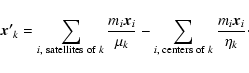
subset as the "centers'' of the orbit. For each orbit k, we define
with a convenient
choice of origin). It is equivalent to say that we describe our system
with n-1 "orbits'', each one corresponding to the center of mass of
a first subset of the bodies orbiting the center of mass of a second
subset of the bodies. In the following, we shall refer for each orbit
to the first subset as the "satellites'' of the orbit, and to the second
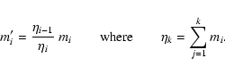
subset as the "centers'' of the orbit. For each orbit k, we define
| |
= | (10) | |
| = | (11) |
We may give a matrix formulation of this transformation. We define
![]() as the n-vector of the barycentric positions of the
bodies, and
as the n-vector of the barycentric positions of the
bodies, and ![]() as the n-vector of the generalized Jacobi
positions. Equation (12) for each k can be viewed as
as the n-vector of the generalized Jacobi
positions. Equation (12) for each k can be viewed as
![]() ,
where M is a fixed
,
where M is a fixed ![]() matrix, defined by
matrix, defined by
| (13) |
 |
(15) |
Hence as for the barycentric coordinates, in the generalized Jacobi
coordinates, the kinetic energy appears as a weighted sum of the squared
momenta
(there are no cross terms of the form
![]() ). It is
equivalent to say that
). It is
equivalent to say that
![]() for each i.
This property is the cornerstone of our method. It allows the Hamiltonian
to naturally split, as for the MVS method, into a sum of separate
Keplerian Hamiltonians plus a perturbation that does not depend
on the momenta. This is indeed the reason why
Wisdom & Holman (1991) make use of the Jacobi coordinates in the Keplerian part of
their method, even though everything else is computed in heliocentric
coordinates. In their Democratic
Heliocentric method, developed for integrating close encounters,
Duncan et al. (1998) use heliocentric coordinates. In that case, the kinetic
energy does not reduce to such a simple form. It is then necessary
to split the Hamiltonian into three separate parts. This does not cause
big trouble except for orbits with very small perihelia. A special
modification of the method has been developed in Levison & Duncan (2000) to
overcome this difficulty.
for each i.
This property is the cornerstone of our method. It allows the Hamiltonian
to naturally split, as for the MVS method, into a sum of separate
Keplerian Hamiltonians plus a perturbation that does not depend
on the momenta. This is indeed the reason why
Wisdom & Holman (1991) make use of the Jacobi coordinates in the Keplerian part of
their method, even though everything else is computed in heliocentric
coordinates. In their Democratic
Heliocentric method, developed for integrating close encounters,
Duncan et al. (1998) use heliocentric coordinates. In that case, the kinetic
energy does not reduce to such a simple form. It is then necessary
to split the Hamiltonian into three separate parts. This does not cause
big trouble except for orbits with very small perihelia. A special
modification of the method has been developed in Levison & Duncan (2000) to
overcome this difficulty.
With the kinetic energy expressed as in Eq. (14), we may now
split the Hamiltonian (3) as
Both methods have distinct application
fields. In the Solar System, there is only a factor
![]() 2 between two successive planetary orbits. The stability of
the system is ensured by the mass of the Sun. Hence the MVS method
is well suited in this case. In hierarchical stellar
systems, there is no dominant mass, but the scaling factor between
successive orbits is usually much larger than 2.
2 between two successive planetary orbits. The stability of
the system is ensured by the mass of the Sun. Hence the MVS method
is well suited in this case. In hierarchical stellar
systems, there is no dominant mass, but the scaling factor between
successive orbits is usually much larger than 2.
Our symplectic method is entirely based on this splitting of the Hamiltonian. In fact, this is the natural splitting of generalized Jacobi variables. As a result, we call our method the Hierarchical Jacobi Symplectic (HJS).
A special case arises if we add some massless particles, usually called "test particles''. In a stellar system, the hierarchical structure is defined from the relative orbits of the massive bodies. Adding one test particle means adding a body, but also an orbit. The "satellites'' of this orbit reduce to the particle itself, but the centers, i.e., the subset of bodies the particle is intended to orbit around, must be specified. Moreover, even if this new massless body does not affect the massive ones, the new orbit must follow the hierarchical structure of the system. In practice, this means that the test particle has to be added to the list of centers or satellites of some outer orbits. This of course does not affect the dynamics of the other bodies, but does for the particle itself. It adds some terms to the second order equations derived from HB (and used in the code) that define the perturbing acceleration on the particle. For example, we consider the double-binary system in which we want to add a circumbinary disk of test particles orbiting one of the binaries. Each of these particles will be considered as orbiting the center of mass of that binary, but it must be considered as an additional center for the relative orbit between the two binaries, otherwise the hierarchical rules are not fulfilled. Of course this does not affect the dynamics of the outer orbit, but in practice, this adds a term to the dynamics of each particle.
In the following, we apply the HJS method in various situations
of astrophysical interest relevant to the dynamics of multiple
stellar systems. The HJS method applies indeed to a large variety
of situations. The limitations of the
method are those that ensure the condition
![]() :
i) close
encounters must be avoided, ii) the hierarchy must not change: a given
particle orbiting a subset of centers must keep orbiting around
the same centers during the computation. In the runs we describe
below, these conditions are not strictly speaking respected for the test
particles, as gravitational perturbations may
cause a lot of particles to escape from the
system. However, we are mainly interested in those particles that
remain in the system. The fact that the dynamics of the particles
that escape are not computed with great accuracy at ejection time does
not affect our conclusion, the important thing being that
the particles initially located at some locations in the system are
actually unstable, irrespective of their dynamics at ejection time.
:
i) close
encounters must be avoided, ii) the hierarchy must not change: a given
particle orbiting a subset of centers must keep orbiting around
the same centers during the computation. In the runs we describe
below, these conditions are not strictly speaking respected for the test
particles, as gravitational perturbations may
cause a lot of particles to escape from the
system. However, we are mainly interested in those particles that
remain in the system. The fact that the dynamics of the particles
that escape are not computed with great accuracy at ejection time does
not affect our conclusion, the important thing being that
the particles initially located at some locations in the system are
actually unstable, irrespective of their dynamics at ejection time.
Designing accurate tests for the HJS method is not a straightforward task, as there is virtually no typical behavior for multiple stellar systems, each configuration being in itself a peculiar case. There are basically three kinds of features that can be tested:
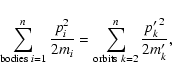
The most straightforward test is to investigate for any integration the stability of the global energy and of the angular momentum of the system over the integration time. Note that this test is relevant only if more than two massive bodies are present, independent of the number of test particles. If this is not the case, then the relative orbit between the two bodies is fixed, and the method solves it obviously to machine precision.
![\begin{figure}
\includegraphics[angle=-90,width=8cm,clip]{ms3133f2}\end{figure}](/articles/aa/full/2003/12/aa3133/img200.gif) |
Figure 1:
Dynamical evolution of a circumbinary disk orbiting a
binary with mass parameter |
| Open with DEXTER | |
Second, any integration can be performed in parallel with a more conventional, and more CPU-time consuming integrator like the Burlish & Stoer method. However the comparison will be of interest only over rather short time spans, as the Burlish & Stoer method is not symplectic.
Third, there are some known results concerning peculiar dynamical situations that we aim to reproduce (but more rapidly) with the HJS integrator. We must obtain stability when it is expected. This may concern test particles (e.g., gaps in circumbinary disks), or the massive bodies themselves, such as the Kozai resonance in triple systems. This will constitute our guideline for the following tests.
Many young stellar systems were observed in recent years to harbor dusty or gaseous disks orbiting a binary star. These disks are today known as circumbinary disks. This includes the examples of GG Tauri (Guilloteau et al. 1999; White et al. 1999), UY Ori (Duvert et al. 1998; Close et al. 1998), and HD 98800 (Koerner et al. 2000). Circumbinary disks are known to be cleared from inside by interaction with the components of the binary, leading to a sharp inner edge located well outside the orbit of the central binary. There is observational evidence for this fact (Guilloteau et al. 1999), and this was predicted by many theoretical studies, often using smoothed particle hydrodynamics (SPH) (Artymowicz & Lubow 1994; Artymowicz & Lubow 1996; Bate 2000). All these simulations show that the inner gap of the disk opens within a few orbital periods of the binary, with spiral density waves extending far in the remaining disk. Artymowicz & Lubow (1996) show that some of the tidally eroded mass can flow towards the individual stars by so-called "streamers''.
Trying to reproduce these characteristics is a valuable test for the HJS integrator. In fact, a circumbinary disk can still be simulated with the standard MVS integrator if we give the test particles the higher indexes. One of the two stars needs to be taken as the "sun'', the other one being a "perturber''. This still works because there are here only two massive bodies; their mutual orbit is then left unchanged and is solved exactly independent of the method. However we must assume that the dominant Keplerian motion of the test particles is around the "sun'' chosen for the system. Hence the perturbation arising from the other star is comparable to the dominant Keplerian motion, but it still works because we adopt a time-step of 1/20 of the smallest orbital period, i.e., that of the binary, which represents a much smaller fraction of the orbital periods of the test particles.
However, the orbital motion of test particles in a circumbinary disk is usually described with respect to the center of mass of the binary, which is exactly the framework of the HJS method. As a matter of fact, the HJS formulation appears much more natural for such a system. In an HJS integration, the circumbinary disk is simulated as a set of test particles orbiting the center of mass of a binary star (to which is given the total mass of the binary), and perturbed by each component. The main goal is to reproduce the inner gap clearing phase, in both size and shape. We nevertheless do not expect to properly simulate the streamers onto the central stars, as whenever particles fall in between the two stars, or close to one of them, it can hardly be regarded as mainly orbiting the center of mass of the system. As the particles do not interact with each other, we cannot give any viscosity to the disk, contrary to SPH integrations. However, with respect to SPH simulations, we are able to take many more particles in the disk, and to integrate the dynamics of the disk over a much longer time span, which allows us to investigate the relaxation of the disk and the dissipation of the spiral density waves.
Dynamically speaking, a binary system is characterized by an orbital
eccentricity e and by a mass parameter ![]() :
the masses of the stars
are
:
the masses of the stars
are ![]() and
and ![]() where M is the total mass. The semi-major
axis a of the binary does not need to be specified, as the whole
problem (gap sizes, evolution time-scale) just rescales with a.
Figure 1 shows the evolution of the gap for a disk
orbiting a binary with (e=0.1,
where M is the total mass. The semi-major
axis a of the binary does not need to be specified, as the whole
problem (gap sizes, evolution time-scale) just rescales with a.
Figure 1 shows the evolution of the gap for a disk
orbiting a binary with (e=0.1, ![]() ), as computed with the HJS2
(second order) integrator. All distances are given
relative to a. The initial disk holds 105 particles located
between r=1.5a and r=3.5a from the center of mass of the system,
with a surface density
), as computed with the HJS2
(second order) integrator. All distances are given
relative to a. The initial disk holds 105 particles located
between r=1.5a and r=3.5a from the center of mass of the system,
with a surface density ![]() r-1. Note that the inner edge of the
initial disk is far inside the expected size of the gap, so that it has
no influence on the result.
r-1. Note that the inner edge of the
initial disk is far inside the expected size of the gap, so that it has
no influence on the result.
![\begin{figure}
\includegraphics[angle=-90,width=8cm,clip]{ms3133f2}\end{figure}](/articles/aa/full/2003/12/aa3133/img74.gif) |
Figure 2:
Approximate radius of the inner edge of the circumbinary disk
as computed with HJS integrations, in units of the semi major axis a of the binary, for various values of e and |
| Open with DEXTER | |
Figure 1 must be compared to Fig. 9 from Artymowicz & Lubow (1994) which displays the evolution of a similar system, computed with SPH. We see in Fig. 1 that we reproduce the gap clearing phase, the spiral density waves and even the streamers. However, we may not trust the dynamics of the particles once they have fallen between the two stars. This does not matter, as in any case, these particles are rapidly removed from the system (or accreted by the stars). The final gap is at r=2.6a, consistent with the simulations of Artymowicz & Lubow (1994).
The time-step used in our simulation is 1/20 of the orbital period of the binary. This is a classical choice for MVS-like integrators. Any other, non-symplectic integrator would need to use a time-step at least 50 times less to get the same result. As a matter of fact, we were able to carry out the integration up to 105 orbital periods (this took approximatively 1 day of CPU-time), which is not possible with SPH. At t=105, the gap is totally cleared, and the sharp inner edge of the disk clearly shows up. In fact, at this time, the remaining circumbinary disk is fully stable and relaxed. The disk does no longer lose particles. Actually the gap clearing is almost achieved after a few hundred periods.
We performed several simulations of the same kind, for various sets
of values ![]() .
The results are summarized in Fig. 2
which displays the size of the computed inner gap of the circumbinary
disk as a function of the eccentricity e, for two values of
.
The results are summarized in Fig. 2
which displays the size of the computed inner gap of the circumbinary
disk as a function of the eccentricity e, for two values of ![]() .
The size of the gap is appreciated after 300 orbital periods of the
binary. The result are consistent with the corresponding figures
from Artymowicz & Lubow (1994). We note as expected a gradual increase of the gap
as a function of the eccentricity, and on average a larger gap for
a larger
.
The size of the gap is appreciated after 300 orbital periods of the
binary. The result are consistent with the corresponding figures
from Artymowicz & Lubow (1994). We note as expected a gradual increase of the gap
as a function of the eccentricity, and on average a larger gap for
a larger ![]() .
The sudden increase of the gap when reaching
.
The sudden increase of the gap when reaching
![]() is due to the 4:1 commensurability that falls at
r=2.52a. This commensurability always clears a ring-like
additional gap; whenever the inner edge of the disk gets close to this
gap, it merges with it, leading to a sudden increase of the central gap.
is due to the 4:1 commensurability that falls at
r=2.52a. This commensurability always clears a ring-like
additional gap; whenever the inner edge of the disk gets close to this
gap, it merges with it, leading to a sudden increase of the central gap.
![\begin{figure}
\includegraphics[angle=-90,width=8cm,clip]{ms3133f2}\end{figure}](/articles/aa/full/2003/12/aa3133/img201.gif) |
Figure 3: Dynamical evolution of the same system as in Fig. 1, but to which two circumstellar disks orbiting the individual stars have been added. The plotting conventions are the same as for Fig. 1. |
| Open with DEXTER | |
Apart from a circumbinary disk, a binary star can also harbor
circumstellar disks orbiting each of its components. Of course
we expect these disks, if present, to be tidally truncated outwards.
This is what is actually observed in the HK Tauri
system (Koresko 1998; Stapelfeldt et al. 1998). In this system, the secondary star was
observed to be surrounded by a circumstellar disk, almost seen edge-on
from the Earth. This disk is probably tidally truncated by the
primary, as it extends to ![]() 1/3 of the projected separation of the
two stars Stapelfeldt et al. (1998).
1/3 of the projected separation of the
two stars Stapelfeldt et al. (1998).
In order to further test the HJS method, we added to the previous simulation two circumstellar disks of particles orbiting each individual star. More precisely, we still take 105 particles, but we leave 50 000 of them in the circumbinary dusk, and put 25 000 in two circumstellar disks orbiting each star. The circumstellar disks are initially chosen identical, with an initial outer radius of 0.7a. These disks are assumed for simplicity to be coplanar with the binary orbit and the circumbinary disk, but inclined disks, as this seems to be the case for HK Tauri (Koresko 1998), could be easily simulated. Note that such a configuration can no longer be simulated with the MVS method, as now all particles do not orbit the same massive center.
Figure 3 displays two snapshots of that simulation, at t=0.5 orbital period of the binary, and t=100 periods. In the first snapshot, we clearly see the tidal erosion of the outer edges of the individual disks. The sculpting of the inner edge of the circumbinary disk is the same as in Fig. 2. In the second snapshot, the disks have stabilized. We see the sharp truncation of the disks. As expected, the disk surrounding the secondary star is smaller than the one orbiting the primary star (recall that the disks were initially identical). The remaining disks do not exhibit any strong tidal perturbation by the companion star, as this seems to be also the case for HK Tauri (Koresko 1998).
Hierarchical triple systems consist usually of three bodies of comparable masses, the distance between two of them being much smaller than their distance to the third body. In a first approximation, the dynamics of such a system can be regarded as two nested Keplerian orbits, the first one involving a close binary (the two first bodies), and the second one describing the third body orbiting the center of mass of the close binary. We shall hereafter refer the orbit of the close binary as the inner orbit, and the orbit of the third body as the outer orbit.
Of course, in the framework of the HJS formalism, this description with two fixed orbits corresponds exactly to the Hamiltonian HA given by Eq. (16), and the two orbits themselves correspond to the Jacobi coordinates introduced above. Due to the perturbing Hamiltonian HB (Eq. (17)), the two orbits are slowly modified. We expect the HJS integrator to efficiently compute this secular evolution. Here again, the MVS integrator can still work for such a system, because the description of the inner orbit is the same in both formulations. The outer orbit is however not described identically in both method, but as the time-step is fixed by the inner one, resulting in a very small fraction of the outer orbital period, the dynamics of the third body can still be computed with the MVS technique, but less safely than if we adopt the more natural hierarchical formulation of HJS.
The global behavior of such triple systems has been the subject of several theoretical investigations in the past 30 years (Harrington 1968; Mazeh & Shaham 1977, 1979; Söderhjelm 1984; Krymolowski & Mazeh 1999). First, the semi-major axes of both orbits appear very stable, apart from very small amplitude and short period variations. This is due to the fact that the short period terms rapidly average over a few orbits; second, the outer orbit appears very stable, apart from a slow precession of the line of apsides. The most striking fact concerns the evolution of the inner orbit. Despite a constant semi-major axis, its eccentricity can be subject to large modulations, even if the orbit is initially circular, the main parameter controlling this being the mutual inclination between the two orbits. This was initially described by Harrington (1968), Mazeh & Shaham (1977, 1979), and Söderhjelm (1982).
A full numerical and semi-analytical study is given in Krymolowski & Mazeh (1999).
Here we aim to reproduce their results using the HJS integrator.
In order to make the comparison possible, we then assume the same
initial conditions as them, i.e. a mass ratio
![]() between the two components of the inner binary, and similarly
between the two components of the inner binary, and similarly
![]() for the third body; the period ratio
between the two orbits is fixed to 28. This leads to a semi-major
axis ratio
for the third body; the period ratio
between the two orbits is fixed to 28. This leads to a semi-major
axis ratio
![]() .
The initial eccentricities of the orbits
are fixed initially to
.
The initial eccentricities of the orbits
are fixed initially to
![]() and
and
![]() ,
and the longitude of periastron of the outer orbit with respect to
the periastron of the inner orbit is fixed initially to
,
and the longitude of periastron of the outer orbit with respect to
the periastron of the inner orbit is fixed initially to
![]() .
.
![\begin{figure}
\par\includegraphics[angle=-90,width=8.8cm,clip]{ms3133f4}\end{figure}](/articles/aa/full/2003/12/aa3133/img84.gif) |
Figure 4:
Evolution of the eccentricity
|
| Open with DEXTER | |
Defined this way, our problem is scale-invariant. Our time basis will
the orbital period of the inner orbit. As usual in HJS and MVS runs,
we first fix the time-step to 1/20 of that time basis.
The main parameter we wish to describe here
is the eccentricity of the inner orbit, as a function of the mutual
inclination between the two orbits, as this is the most critical
evolution. Figure 4 shows this evolution, as computed
with the HJS2 integrator over
![]() revolutions of the inner orbit,
for an initial mutual inclination of
revolutions of the inner orbit,
for an initial mutual inclination of
![]() .
It can be directly
compared to the corresponding integration with the same initial
parameters given in Fig. 2 from Krymolowski & Mazeh (1999) (We only display
the evolution over
.
It can be directly
compared to the corresponding integration with the same initial
parameters given in Fig. 2 from Krymolowski & Mazeh (1999) (We only display
the evolution over
![]() revolution instead of
revolution instead of
![]() in order
to better visualize the evolution). Figure 4 appears virtually
identical to their direct integration of Newton's equations with
a Burlish & Stoer method. We confirm that for such moderate inclinations,
the eccentricity of the inner orbit is subject to a superposition of
two modulations: a large amplitude, long-term one
(period
in order
to better visualize the evolution). Figure 4 appears virtually
identical to their direct integration of Newton's equations with
a Burlish & Stoer method. We confirm that for such moderate inclinations,
the eccentricity of the inner orbit is subject to a superposition of
two modulations: a large amplitude, long-term one
(period ![]() 380 inner revolutions), and a smaller amplitude,
more rapid one (period
380 inner revolutions), and a smaller amplitude,
more rapid one (period ![]() 80 inner revolutions). The mutual
inclination i, initially fixed at
80 inner revolutions). The mutual
inclination i, initially fixed at
![]() ,
appears to rapidly
fluctuate around this value with an amplitude less than
,
appears to rapidly
fluctuate around this value with an amplitude less than
![]() ,
so twe do not display it here.
,
so twe do not display it here.
We get the same result as the direct integration by Krymolowski & Mazeh (1999), thus confirming the validity of the HJS integration. However, the main difference is that we use here a very large time-step compared to the one needed for direct integrations. As a consequence, it only takes us a few minutes of CPU time to perform the integration, compared to several hours with direct methods.
![\begin{figure}
\par\includegraphics[width=8.8cm,clip]{3133f5.eps}\par\end{figure}](/articles/aa/full/2003/12/aa3133/img210.gif) |
Figure 5: Relative energy error with respect to the initial value as a function of time, for the integration corresponding to Fig. 4, in the cases of the use of the HJS2 integrator (black) and of the HJS4 integrator (grey). |
| Open with DEXTER | |
![\begin{figure}
\par\includegraphics[angle=-90,width=8.8cm,clip]{ms3133f6}\end{figure}](/articles/aa/full/2003/12/aa3133/img89.gif) |
Figure 6:
Maximum relative energy error over several integrations
of the triple system with
|
| Open with DEXTER | |
As a further confirmation, we also perform the same integration with
the HJS4 (fourth order) integrator. We do not display here the corresponding
result for the evolution of
![]() ,
as it appears to exactly
match Fig. 4. It is more interesting to check the energy
preservation. Checking energy preservation was of no use in our
circumbinary disk
test, as the two massive bodies moved on a fixed orbit. Conversely, this
is here of interest, as we have three massive bodies.
Figure 5 shows the relative energy error with respect
to the initial value, as a function of time, for the two (HJS2 and HJS4)
integrations. In the HJS2 run, it appears to range between 10-9and a few 10-5, which is equivalent to what Krymolowski & Mazeh (1999) get in
their integrations. In the HJS4 integration, the relative energy
error now remains
,
as it appears to exactly
match Fig. 4. It is more interesting to check the energy
preservation. Checking energy preservation was of no use in our
circumbinary disk
test, as the two massive bodies moved on a fixed orbit. Conversely, this
is here of interest, as we have three massive bodies.
Figure 5 shows the relative energy error with respect
to the initial value, as a function of time, for the two (HJS2 and HJS4)
integrations. In the HJS2 run, it appears to range between 10-9and a few 10-5, which is equivalent to what Krymolowski & Mazeh (1999) get in
their integrations. In the HJS4 integration, the relative energy
error now remains ![]() 10-6, for a roughly doubled computing
time with respect to the HJS2 integration.
10-6, for a roughly doubled computing
time with respect to the HJS2 integration.
Additional checking can be achieved if we now let the time-step vary.
This is illustrated in Fig. 6, which displays the maximum
relative energy error quoted over the
![]() inner revolution
integrations, for various time-steps and with both integrators, in logarithmic
scale. As a matter of fact, we get a slope close to 2 for the HJS2
integrator, and close to 4 for the HJS4 integrator.
inner revolution
integrations, for various time-steps and with both integrators, in logarithmic
scale. As a matter of fact, we get a slope close to 2 for the HJS2
integrator, and close to 4 for the HJS4 integrator.
![\begin{figure}
\par\includegraphics[angle=-90,width=8.8cm,clip]{ms3133f7}\end{figure}](/articles/aa/full/2003/12/aa3133/img90.gif) |
Figure 7:
Same as Fig. 4, but for an initial mutual
inclination
|
| Open with DEXTER | |
![\begin{figure}
\par\includegraphics[angle=-90,width=8.8cm,clip]{ms3133f8}\end{figure}](/articles/aa/full/2003/12/aa3133/img91.gif) |
Figure 8:
Evolution of the mutual inclination i for the run corresponding
to Fig. 7. The inclination is subject to strong changes in phase
with those of
|
| Open with DEXTER | |
Figure 7 displays the evolution of
![]() under the same
conditions as Fig. 4, but with an initial inclination
under the same
conditions as Fig. 4, but with an initial inclination
![]() .
It can again be directly compared to the corresponding figure (Fig. 4)
from Krymolowski & Mazeh (1999). It exactly matches their direct integration of
Newton's equation.
.
It can again be directly compared to the corresponding figure (Fig. 4)
from Krymolowski & Mazeh (1999). It exactly matches their direct integration of
Newton's equation.
The secular evolution of
![]() is here very different from the
is here very different from the
![]() case. The inner eccentricity is subject to drastic changes
that bring it periodically as high as
case. The inner eccentricity is subject to drastic changes
that bring it periodically as high as ![]() 0.7. Figure 8
shows the corresponding evolution of the mutual inclination ibetween the two orbits. Contrary to the
0.7. Figure 8
shows the corresponding evolution of the mutual inclination ibetween the two orbits. Contrary to the
![]() case, i is
not stable here. It periodically drops down to
case, i is
not stable here. It periodically drops down to ![]()
![]() ,
and
these events appear in phase with the high
,
and
these events appear in phase with the high
![]() episodes.
episodes.
This behavior is actually not surprising; obtaining it is in fact a
validity test for the HJS method. It is known as the Kozai
Resonance, initially described by Kozai (1962) for comets
in the Solar System. In the Solar System, it concerns bodies with initial
high inclinations
and moderate eccentricities with respect to the mid-plane of the Solar System.
Under the effect of secular planetary perturbations (mainly arising from
Jupiter), the orbit is subject to an evolution that drives it periodically
to lower inclination but very high eccentricity,
the semi-major axis remaining constant. The combined evolution of
inclination and eccentricity is due to the secular conservation
of the vertical component of the orbital angular momentum
![]() (thanks to rotational invariance).
Hence if i decreases, then e must increase to keep
(thanks to rotational invariance).
Hence if i decreases, then e must increase to keep ![]() constant.
This periodic evolution is characterized by stopping of the precession rate
of the argument of perihelion
constant.
This periodic evolution is characterized by stopping of the precession rate
of the argument of perihelion ![]() ,
which librates around
,
which librates around
![]() or
or
![]() .
As pointed out by Bailey et al. (1992), this mechanism
is responsible for the origin of most Sun-grazer comets in our Solar
System, in particular those of the Kreutz group.
.
As pointed out by Bailey et al. (1992), this mechanism
is responsible for the origin of most Sun-grazer comets in our Solar
System, in particular those of the Kreutz group.
The Kozai resonance is due to the secular part of the interaction
Hamiltonian of the restricted circular three-body system
(see diagrams in Kozai 1962). It is therefore very generic and is
active as soon as one perturbing planet is present.
The behavior reported in Figs. 7 and 8
is actually a Kozai
resonance, although it concerns here a general (unrestricted)
three-body system. Harrington (1968) first claimed that such a mechanism
should be expected in a hierarchical three-body system with high mutual
inclination, and Söderhjelm (1982) showed that it is active as soon as
![]() .
.
In cometary dynamics, the Kozai resonance modifies the orbit of the particle, not that of the perturbing planet. It can appear surprising that here only the inner orbit is affected. As pointed out in Beust et al. (1997), the more affected orbit in the Kozai resonance is always the one with the smaller angular momentum. Here the angular momentum of the outer orbit is larger than that of the inner orbit.
This evolution
may have some important observational outcomes. Some systems have indeed
been observed with a significant eccentricity of the short-period
inner binary, while it should have been circularized a long time ago
(Mazeh 1990). In the most extreme cases, the eccentricity increase
of the inner orbit could lead to a collision between its two
stellar components, and thus to an instability of the system.
However, for short period binaries, tidal effects between the
components of the inner binary can severely dampen the modulation
of
![]() ,
thus stabilizing the system (Söderhjelm 1984; Beust et al. 1997).
,
thus stabilizing the system (Söderhjelm 1984; Beust et al. 1997).
![\begin{figure}
\par\includegraphics[angle=-90,width=8.8cm,clip]{ms3133f9}\end{figure}](/articles/aa/full/2003/12/aa3133/img99.gif) |
Figure 9: Evolution of the inner eccentricity of the TY Cra system (without tidal effects) as computed with the HJS integrator. A strong Kozai resonance is visible. |
| Open with DEXTER | |
As an extreme application case of this dynamical evolution, Fig. 9
displays the evolution of
![]() for the TY Coronae Australis
(TY Cra) system. This system consists of a central, close
eclipsing binary (semi-major axis 0.066 AU; masses 3.0 and
for the TY Coronae Australis
(TY Cra) system. This system consists of a central, close
eclipsing binary (semi-major axis 0.066 AU; masses 3.0 and
![]() )
surrounded by a tertiary component (
)
surrounded by a tertiary component (![]()
![]() )
orbiting the
binary at
)
orbiting the
binary at ![]() 1.5 AU (Corporon et al. 1996). The mutual inclination
between the two orbits is close to
1.5 AU (Corporon et al. 1996). The mutual inclination
between the two orbits is close to
![]() .
In Beust et al. (1997),
we investigated the dynamics of this system, showing that a strong
Kozai resonance should be expected if no tidal effect was active within the
inner binary. This is actually confirmed by Fig. 9, which
shows the secular evolution of
.
In Beust et al. (1997),
we investigated the dynamics of this system, showing that a strong
Kozai resonance should be expected if no tidal effect was active within the
inner binary. This is actually confirmed by Fig. 9, which
shows the secular evolution of
![]() under such conditions.
We note a drastic Kozai resonance, the peak eccentricity being
under such conditions.
We note a drastic Kozai resonance, the peak eccentricity being
![]() 0.9956! Meanwhile, the mutual inclination i is subject
to sharp drops by more than
0.9956! Meanwhile, the mutual inclination i is subject
to sharp drops by more than
![]() .
It is worth noticing that
even in such extreme cases the HJS integrator is still efficient:
the maximum relative energy error during the eccentricity peaks does
not exceed a few 10-4. This is nevertheless larger than in
Fig. 5, but still acceptable.
.
It is worth noticing that
even in such extreme cases the HJS integrator is still efficient:
the maximum relative energy error during the eccentricity peaks does
not exceed a few 10-4. This is nevertheless larger than in
Fig. 5, but still acceptable.
Rauch & Holman (1999) note that MVS-like algorithms may present some instability when handling very eccentric orbits, with relative energy errors that can reach unity! Even if our energy error still remains significantly smaller, our integration suffers presumably suffers here from a similar instability. Some regularization techniques are given by Rauch & Holman (1999) and could be tested in the present case, be we did not investigate this question as it is beyond the scope of the present paper.
![\begin{figure}
\par\mbox{\includegraphics[width=8.8cm,clip]{ms3133f10a}\hspace*{...
...3f10c}\hspace*{3mm}\includegraphics[width=8.8cm,clip]{ms3133f10d} }
\end{figure}](/articles/aa/full/2003/12/aa3133/img400.gif) |
Figure 10:
Upper view of the four-body GG Tau system with its
circumbinary
disk, as simulated with the HJS integrator. The first plot a)
shows the initial disk together with the four stars and the wide orbit.
The following plots show the evolution of the system after b)
44 000 yr, i.e., after the first periastron passage between the two
binaries, after c)
|
| Open with DEXTER | |
GG Tauri (GG Tau) is a prototype example of a young, pre-main sequence
multiple stellar system. It is located at 140 pc and consists of a
close (![]() 0.3'') central
binary, and of a more distant pair (
0.3'') central
binary, and of a more distant pair (![]() 1.4'') located
1.4'') located
![]() to the south (Guilloteau et al. 1999). Whether these two
binaries are actually gravitationally bound is still an open question,
but it is
highly probable. From combined dynamic and photometric studies
it was possible to constrain the masses of the individual components
of this system: the central binary is more massive
(
to the south (Guilloteau et al. 1999). Whether these two
binaries are actually gravitationally bound is still an open question,
but it is
highly probable. From combined dynamic and photometric studies
it was possible to constrain the masses of the individual components
of this system: the central binary is more massive
(![]() 0.6 and
0.6 and ![]()
![]() )
than the outer one
(
)
than the outer one
(![]() 0.12 and
0.12 and ![]()
![]() )
(White et al. 1999; Simon et al. 2000).
Actually nearly all characteristics of the orbit of the inner binary can be
deduced from the observations (Roddier et al. 1996), while for the two other
orbits (the orbit of the outer binary and the mutual orbit between the
two binaries) only spatial separations can be deduced.
)
(White et al. 1999; Simon et al. 2000).
Actually nearly all characteristics of the orbit of the inner binary can be
deduced from the observations (Roddier et al. 1996), while for the two other
orbits (the orbit of the outer binary and the mutual orbit between the
two binaries) only spatial separations can be deduced.
The central binary is now well known to be surrounded by a dusty and gaseous circumbinary disk that was proved to be in Keplerian rotation around it. As expected for a circumbinary disk, the disk is truncated inwards, with a very sharp inner edge at 180 AU. More surprisingly, the disk also appears somehow truncated outwards. Actually, the dust data reveal that almost 70% of the material is confined in a sharp edged ring-like structure extending between 180 and 260 AU, while the CO data show that the rest of the material extends up to 800 AU or more (Guilloteau et al. 1999).
From a dynamical point of view, the inward truncation of the disk is obviously due to a classical interaction with the central binary like the one we described above, the location of the inner edge appearing as a constraining parameter to the orbit of the binary. The outer shape appears more puzzling to interpret, but it is tempting to attribute it to an interaction with the outer binary. This issue needs nevertheless to be more precisely addressed; the HJS integrator appears indeed well suited for that.
This study will be the subject of a forthcoming paper (Beust & Dutrey 2003).
We may nevertheless summarize here a few results. Figure 10
first shows one evolution of the system over
![]() yrs. In this
simulation, the four massive bodies were given their corresponding
masses, and the orbits were chosen in order to match at t=0 the presently
observed conditions. Of course there were free parameters, but the
major ones are the periastron value q of the mutual orbit between the
two binaries, and the inclinations i and i' between that orbit and
those of the individual binaries (i with respect to the inner binary
and i' with the outer one). The evolution displayed in Fig. 10
corresponds to q=833 AU,
yrs. In this
simulation, the four massive bodies were given their corresponding
masses, and the orbits were chosen in order to match at t=0 the presently
observed conditions. Of course there were free parameters, but the
major ones are the periastron value q of the mutual orbit between the
two binaries, and the inclinations i and i' between that orbit and
those of the individual binaries (i with respect to the inner binary
and i' with the outer one). The evolution displayed in Fig. 10
corresponds to q=833 AU,
![]() and
and
![]() .
The disk is
simulated as 50 000 test particles initially chosen orbiting the
central binary between 150 and 1200 AU, i.e.,
much wider than the observed disk. With these
parameters, the gravitational pull between the binaries at each periastron
passage progressively sculpts the disks and finally the residual disk
appears very close to the observed one. This will be fully detailed
in Beust & Dutrey (2003). Of course the evolution depends on the initial
orbital parameters. If q is too small, the disk is entirely
destroyed, and if it is too large, the remaining disk is too thick
to match the observation; if i is large, we initiate a Kozai
resonance between the orbit of the inner binary and the wide orbit.
This evolution brings the eccentricity of the inner binary to large
values, and this erodes the disk from inside much further out
than the observed 180 AU inner edge.
.
The disk is
simulated as 50 000 test particles initially chosen orbiting the
central binary between 150 and 1200 AU, i.e.,
much wider than the observed disk. With these
parameters, the gravitational pull between the binaries at each periastron
passage progressively sculpts the disks and finally the residual disk
appears very close to the observed one. This will be fully detailed
in Beust & Dutrey (2003). Of course the evolution depends on the initial
orbital parameters. If q is too small, the disk is entirely
destroyed, and if it is too large, the remaining disk is too thick
to match the observation; if i is large, we initiate a Kozai
resonance between the orbit of the inner binary and the wide orbit.
This evolution brings the eccentricity of the inner binary to large
values, and this erodes the disk from inside much further out
than the observed 180 AU inner edge.
i' values around
![]() (i.e. a retrograde orbit for the outer binary with respect to the
mutual orbital motion) appear to be the only range of values that
ensures the stability of the orbit of the outer binary.
It can be seen in Fig. 10 that the separation between the
components of the outer binary is not small compared to the size
(and the periastron) of the wide orbit. Hence the basic hypothesis
of hierarchical motion is marginally fulfilled. This may result in
an instability of the outer binary, its orbit possibly being tidally
disrupted. The HJS integrations revealed that retrograde orbits for
the outer binary are much more stable than prograde and perpendicular
ones. This comes from the fact that if the orbit
is retrograde, then at each periastron passage between the two binaries,
the orbital motion between the two components of the outer binary
is observed to be more rapid from the inner binary. Consequently
the perturbations are better averaged over the orbital motions,
and the whole system is more stable.
In the opposite limiting case (prograde orbit), the outer binary is
close to synchronous revolution of its orbital motion with respect
to the inner binary at each periastron passage. The tidal pull is
subsequently very strong and the outer binary is unstable.
(i.e. a retrograde orbit for the outer binary with respect to the
mutual orbital motion) appear to be the only range of values that
ensures the stability of the orbit of the outer binary.
It can be seen in Fig. 10 that the separation between the
components of the outer binary is not small compared to the size
(and the periastron) of the wide orbit. Hence the basic hypothesis
of hierarchical motion is marginally fulfilled. This may result in
an instability of the outer binary, its orbit possibly being tidally
disrupted. The HJS integrations revealed that retrograde orbits for
the outer binary are much more stable than prograde and perpendicular
ones. This comes from the fact that if the orbit
is retrograde, then at each periastron passage between the two binaries,
the orbital motion between the two components of the outer binary
is observed to be more rapid from the inner binary. Consequently
the perturbations are better averaged over the orbital motions,
and the whole system is more stable.
In the opposite limiting case (prograde orbit), the outer binary is
close to synchronous revolution of its orbital motion with respect
to the inner binary at each periastron passage. The tidal pull is
subsequently very strong and the outer binary is unstable.
As a final test for the HJS integrator, we briefly investigate here
the dynamics of the remarkable sextuple system Castor
(![]() Gem).
Gem). ![]() Gem itself is a visual binary
(Castor A and B) with a
present angular separation of
Gem itself is a visual binary
(Castor A and B) with a
present angular separation of
![]() .
This corresponds to
a physical separation of
.
This corresponds to
a physical separation of ![]() 58 AU, thanks to the parallax
measurement by Hipparcos
(
58 AU, thanks to the parallax
measurement by Hipparcos
(
![]() mas; Torres & Ribas 2002). The
orbit between Castor A and B is well known (Heintz 1988), with
an orbital period of of 467 yr. Each of these components is itself
a single-lined spectroscopic binary, with orbital periods of a few
days. A more distant, eclipsing binary (Castor C, or YY Gem), is seen
at
mas; Torres & Ribas 2002). The
orbit between Castor A and B is well known (Heintz 1988), with
an orbital period of of 467 yr. Each of these components is itself
a single-lined spectroscopic binary, with orbital periods of a few
days. A more distant, eclipsing binary (Castor C, or YY Gem), is seen
at
![]() .
It is located at the same distance as the rest of
the system, and it is therefore probably bound to the whole system.
YY Gem is a double-lined spectroscopic binary with a period
of 0.814 day. The whole system is thus sextuple.
.
It is located at the same distance as the rest of
the system, and it is therefore probably bound to the whole system.
YY Gem is a double-lined spectroscopic binary with a period
of 0.814 day. The whole system is thus sextuple.
As noted by Torres & Ribas (2002), the individual masses of the six individual components can be deduced from combined observations and modeling. Most of the characteristics of the different orbits constituting the system are also known (Torres & Ribas 2002).
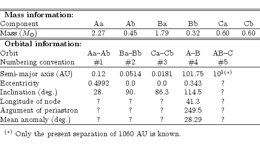 |
The summary of known dynamical information about the Castor system is given in Table 1. These data are extracted from Torres & Ribas (2002) and Heintz (1988), and converted using the Hipparcos parallax. The hierarchical system consists thus of six stars and five orbits. From here on, we adopt the following numbering convention: orbits #1, #2 and #3 will be the internal orbits of binaries A, B and C, respectively. Orbit #4 will be the orbit between Castor A and Castor B, and orbit #5 will be wide orbit between Castor C and the rest of the system (Castor A+B) (see Table 1).
Of course many orbital parameters are still unknown, despite a large
amount of observational data. The best known orbit is
orbit #4, the orbital motion of Castor B with respect to
Castor A, as the motion of both binaries has been now followed for
several tens of years (Heintz 1988). Conversely, the motion of Castor C around Castor A+B (orbit #5) is poorly known, as only a projected
separation of 1060 AU can be inferred. This implies an orbital period
![]() 14 000 yr, which makes it hard to detect orbital motion on a short
time basis.
14 000 yr, which makes it hard to detect orbital motion on a short
time basis.
The HJS integrator may be a well-suited tool for studying the long term dynamics of such a system, as it consists of several orbits of very different sizes. Although a lot of dynamical information is known about the system, there are still many parameters unknown (Table 1), and it is virtually impossible to explore the whole parameter space. As yet, the only global study of the dynamics of the Castor system was made by Anosova et al. (1989) on a statistical trial basis, treating the three binaries as individual point masses. Anosova et al. (1989) concluded nevertheless that the sextuple system was gravitationally bound, and that the wide orbit (orbit #5) was probably eccentric.
Here we want to try to compute the dynamical evolution of the sextuple system, as a final test of the HJS integrator. The test is interesting because the dynamics of the system involves very different time-scales, ranging from less than one day for the orbital motion of the individual binaries to more than 104 yrs for orbit #5. Hence we will need to adopt a small time-step in order to correctly compute orbits #1, 2 and 3, but to carry out the integration over a long enough time basis, in order to see the secular evolution of orbits #4 and #5.
We only describe here one computed evolution as an illustration of the capabilities of the HJS integrator. Exploring the whole parameter space of initial conditions that are not fixed in Table 1 is beyond the scope of the present paper. Hence we take the initial conditions given in Table 1, assuming a semi-major axis of 1060 AU and an eccentricity of 0.5for orbit #5. All other unknown parameters in Table 1 are set to 0.0 at the beginning of the simulation. We expect the most important unknown parameters to be those concerning orbit #5. Depending on the mutual inclination between subsequent orbits, we expect to find Kozai resonances between some of the orbits.
![\begin{figure}
\par\includegraphics[angle=-90,width=8.8cm,clip]{ms3133f11}\end{figure}](/articles/aa/full/2003/12/aa3133/img115.gif) |
Figure 11:
Evolution of the eccentricities of orbit #1, 4 and 5 of the
Castor
system as computed with the HJS integrator. Orbits #2 and 3 are not
shown as their eccentricities remain permanently very low (
|
| Open with DEXTER | |
![\begin{figure}
\par\includegraphics[angle=-90,width=8.8cm,clip]{ms3133f12}\end{figure}](/articles/aa/full/2003/12/aa3133/img116.gif) |
Figure 12: Evolution of the inclinations of all orbits of the Castor system as computed with the HJS integrator. The inclinations are computed with respect to the invariable plane of the whole system (perpendicular to its angular momentum). |
| Open with DEXTER | |
![\begin{figure}
\par\includegraphics[angle=-90,width=8.8cm,clip]{ms3133f13}\end{figure}](/articles/aa/full/2003/12/aa3133/img117.gif) |
Figure 13: Evolution of the mutual inclination of orbit #4 with respect to orbit #5, as computed with the HJS integrator. |
| Open with DEXTER | |
![\begin{figure}
\par\includegraphics[angle=-90,width=8.8cm,clip]{ms3133f14}\end{figure}](/articles/aa/full/2003/12/aa3133/img118.gif) |
Figure 14: Same as Fig. 13, but for the argument of periastron of orbit #4 with respect to the plane of orbit #5, and similarly for orbit #1 with respect to orbit #4. |
| Open with DEXTER | |
The integration we present here was carried out for 106 yrs, using
a time-step of 1/20 of the smallest orbit (#4), i.e. 1 hour. This
took approximatively one week of CPU on a single IBM power3+
processor. The maximum relative energy error over the whole integration
was ![]() 10-7.
10-7.
Figure 11 shows the computed evolution of the orbital eccentricities of orbits #1, 4 and 5. The eccentricities of orbits #2 and 3 remain very small and do not need to be displayed here. Figure 12 shows the evolution of the inclinations of all orbits, as computed with respect to the invariable plane of the whole system.
We first note that orbits #2 and #3 are very stable. Their eccentricities remain very small and their inclinations are not subject to significant changes; these orbits concern Castor B and C, and they are the smallest ones, so that the inner motion of these two binaries is almost independent of the secular motion of the whole system. This is particularly the case for orbit #3. We could have merged Castor C into a single body for the computing of the rest of the dynamics.
This is not the case for orbit #1 (Aa-Ab), which is
wider than orbits #2 and #3, and consequently clearly interacts
with the global motion. The major changes actually concern orbits #4
and #5. We note a periodic modulation of the eccentricity of
orbit #4 together with synchronous changes of the inclinations of
both orbits. There is obviously a Kozai resonance between them. This is
confirmed by Fig. 13 which shows the evolution of the
mutual inclination between the two orbits. As usual, we see in
Fig. 12 that the inner orbit (#4) is more affected by the
outer (#5), especially its eccentricity. This is due to the larger
value of the angular momentum of orbit #5 than of
orbit #4. However, the angular momentum ratio between these two
orbits is only ![]() 2.7, so that orbit #5 is also affected by the
Kozai resonance (Fig. 12).
2.7, so that orbit #5 is also affected by the
Kozai resonance (Fig. 12).
However, with respect to standard behavior in Kozai resonance (see three body simulations above), we note in Figs. 11-13 an additional, higher frequency modulation in the secular evolution of the eccentricities and inclinations of the orbits affected by the Kozai resonance (#4 and #5). This additional modulation is due to the interaction with the inner orbits (mainly orbit #1), as the Kozai resonance reported here concerns three binaries instead of single bodies. Obviously the HJS integrator is very efficient to compute this dynamics.
Orbit #1 (Castor Aa-Ab) is clearly affected by the interaction with
the rest of the system. This is obvious in Figs. 11 and 12, which show significant eccentricity and inclination
changes of that orbit. Despite the fairly large eccentricity
modulation, this orbit is not trapped in a Kozai resonance with
orbit #5, i.e. the outer orbit just above it. This shows up in
Fig. 14, which displays the secular evolution of the
argument or periastron
![]() of orbit #4 with respect to
the plane orbit #5, and that of
of orbit #4 with respect to
the plane orbit #5, and that of
![]() ,
which is the same
for orbit #1 with respect to orbit #4. We note a libration of
,
which is the same
for orbit #1 with respect to orbit #4. We note a libration of
![]() around
around
![]() ,
which is characteristic for a
Kozai resonance. Conversely,
,
which is characteristic for a
Kozai resonance. Conversely,
![]() is subject to a more or less
regular precession, and is thus not confined around a fixed value.
is subject to a more or less
regular precession, and is thus not confined around a fixed value.
Of course this dynamic depends on the initial conditions we choose; we could
actually get different situations if we assumed different values. Exploring
the whole parameter space is nevertheless beyond the scope of the
present paper, as we only want to illustrate applications for the
HJS orbit. We note nevertheless that finding a Kozai resonance between
orbits #4 and #5 may appear not surprising, as the period ratio
between them is ![]() 30. Conversely, the period ratio between
orbits #1 and #4 is
30. Conversely, the period ratio between
orbits #1 and #4 is ![]() 18 500. The typical period of the eccentricity
modulation due to the Kozai resonance is
18 500. The typical period of the eccentricity
modulation due to the Kozai resonance is ![]()
![]() ,
where
,
where
![]() and
and
![]() are the orbital periods
of respectively the outer and inner orbits involved in the Kozai resonance
(Söderhjelm 1982).
For orbits #4 and #5 we derive a period of
are the orbital periods
of respectively the outer and inner orbits involved in the Kozai resonance
(Söderhjelm 1982).
For orbits #4 and #5 we derive a period of
![]() yrs, which
is somewhat shorter but comparable to the one appearing in
Fig. 11. For orbits #1 and #4, the same estimate gives
a period larger than
yrs, which
is somewhat shorter but comparable to the one appearing in
Fig. 11. For orbits #1 and #4, the same estimate gives
a period larger than
![]() yrs, which is far larger than the time-span
of our integration. Actually the shorter period perturbations on that
orbit arising from all components of the system overcome the very long
term Kozai modulation, making
yrs, which is far larger than the time-span
of our integration. Actually the shorter period perturbations on that
orbit arising from all components of the system overcome the very long
term Kozai modulation, making
![]() precess.
precess.
The absence of Kozai resonance between orbits #1 and #4 nevertheless does not prevent orbit #1 from being significantly affected by the six-body system dynamics, while this is not the case for the closer orbits #2 and #3. This may actually explain why orbit #1 is presently eccentric, which is not the case for orbits #2 and #3. These last two orbits may have been tidally circularized, while this is not the case for the wider orbit #1.
The HJS integrator is a modified MVS-like technique that permits the symplectic integration of n-body hierarchical systems with comparable masses. The different application examples described above show that is very well suited for the study of various dynamical configurations, even of high complexity. The gain in computing speed is at least one or two orders of magnitude with respect to conventional techniques where the first order hierarchical Keplerian motion is not built-in. In fact, the gain is comparable to the one provided by the MVS-like integrators designed for planetary system study.
The application examples presented in the present paper do not represent an exhaustive description of all the capabilities of the HJS integrator. There are many other problems to which it could apply, such as for example the dynamics of planets (S or P type) in binary or even multiple stellar systems. There are two major limitations to the HJS technique though. First, close encounters between two bodies are not permitted unless they are the only two members of one of the orbits followed in the integration. This difficulty was already encountered in the MVS technique for the study of the final (violent) stages of formation of planetary systems. Duncan et al. (1998) overcome this difficulty in their SyMBA integrator, but they need to split the Hamiltonian into three parts instead of two, and above all they use heliocentric coordinates, thus particularizing the central body. With the HJS integrator we move in the opposite direction, trying not to particularize any of the massive bodies. Hence the study of planetary system formation in multiple stellar systems could appear problematic with the HJS integrator if close encounters play a significant role. An intermediate technique dedicated to the study of planets in binary systems was recently developed by Chambers et al. (2002). Basically, the coordinates they introduce are almost equivalent to our generalized Jacobi ones, but all planets are treated on the same level. This allows them to handle close encounters, but consequently the Hamiltonian must be split into three parts; if the planetary orbits are treated on the same level, the full hierarchical structure is not respected. The Chambers et al. (2002) technique is identical to ours if only one planet is present in the binary system. If there are many planets, then the third part of the Hamiltonian does not cancel. The major consequence is that the second order acceleration formulas used in the code are much more complex; this renders the generalization to any configuration in a multiple stellar system more difficult. Chambers et al. (2002) use different explicit formulas (and thus different codes) depending whether type S (orbiting one of the two stars) or type P (orbiting the binary) planets are considered. Of course this no longer applies if the stellar system harbors more than two stars. A valuable future evolution of the HJS integration would then be a possible synthesis of HJS and of the Chambers et al. (2002) technique. In order for this to be possible, the various bodies involved in the n-body system should be classified into three subsets instead of two: i) the "stars'', i.e., the most massive bodies whose hierarchical structure must follow the rules defined in the present paper and which cannot undergo close encounters among themselves; ii) the "planets'', i.e., less massive bodies that are supposed to orbit a given center of mass in the stellar system, with no other constraint on the hierarchical structure; iii) massless test particles that would be treated as usual.
Another limitation of the HJS technique is that the hierarchical structure of the system must be preserved along the integration. This is not in itself a very strong constraint, as in any hierarchical n-body system, whenever a Keplerian structure is broken, at least part of the bodies concerned are usually lost by the system within a very short time-scale. Hence even if the final escape motion is not well computed, the final result is the same.
Acknowledgements
All the computations presented in this paper were performed at the Service Commun de Calcul Intensif de l'Observatoire de Grenoble (SCCI).
In the matrix formulation introduced in the text, the kinetic energy can
be written algebraically (with convenient product definition) as
 |
(A.1) |
 |
(A.2) |
 |
(A.3) |
 |
(A.4) |
| B1j | = | 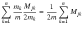 |
|
| = | 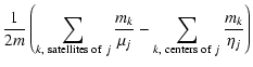 |
||
| = | 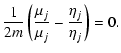 |
(A.5) |
| Bij | = | 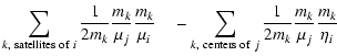 |
|
| = | 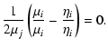 |
(A.6) |
| Bii | = |  |
|
| = | 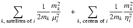 |
||
| = | 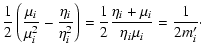 |
(A.7) |
We recall the way we split the Hamiltonian of the n-body problem in the HJS
method.
| HA | = | 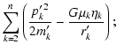 |
(B.1) |
| HB | = | 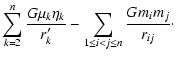 |
(B.2) |
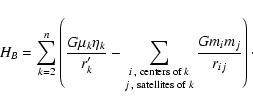 |
(B.3) |
 |
(B.4) |
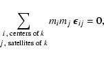 |
(B.5) |
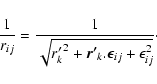 |
(B.6) |
![\begin{displaymath}\frac{1}{r_{ij}}=\frac{1}{r'_k}\left[
1-\frac{1}{2}\frac{\vec...
...}{{r'_k}^2}+O\left(
\frac{\epsilon^2}{{r'_k}^2}\right)\right],
\end{displaymath}](/articles/aa/full/2003/12/aa3133/img157.gif) |
(B.7) |
![\begin{displaymath}% latex2html id marker 407
\includegraphics[width=8.8cm,clip]{equation8.eps}\end{displaymath}](/articles/aa/full/2003/12/aa3133/img220.gif) |
(B.8) |
HJS was built as a superset of the popular SWIFT package (Levison & Duncan 1994). The routines constituting HJS are publicly available via http://www-laog.obs.ujf-grenoble.fr/~beust/hjs.html. They must must be added to the SWIFT package and compiled with it. Instruction for compilation and for running are given via the same URL.