of cool-star atmospheres
A&A 400, 679-694 (2003)
DOI: 10.1051/0004-6361:20021793
L. Decin1,![]() -
B. Vandenbussche1 -
C. Waelkens1 -
K. Eriksson2 -
B. Gustafsson2 -
B. Plez3 -
-
B. Vandenbussche1 -
C. Waelkens1 -
K. Eriksson2 -
B. Gustafsson2 -
B. Plez3 -
A. J. Sauval4 -
K. Hinkle5
1 - Instituut voor Sterrenkunde, KULeuven, Celestijnenlaan 200B, 3001
Leuven, Belgium
2 -
Institute for Astronomy and Space Physics, Box 515, 75120 Uppsala, Sweden
3 -
GRAAL - CC72, Université de Montpellier II, 34095 Montpellier Cedex 5,
France
4 -
Observatoire Royal de Belgique, Avenue Circulaire 3, 1180 Bruxelles,
Belgium
5 -
National Optical Astronomy Observatory![]() , PO Box 26732, Tucson, Arizona 85726, USA
, PO Box 26732, Tucson, Arizona 85726, USA
Received 22 November 2001 / Accepted 2 December 2002
Abstract
The fine calibration of the ISO-SWS detectors (Infrared Space
Observatory - Short Wavelength Spectrometer) has proven to be a
delicate problem. We therefore present a
detailed spectroscopic study in the 2.38-12 ![]() m wavelength range
of a sample of 16 A0-M2 stars used for the calibration of
ISO-SWS. By investigating the discrepancies between the ISO-SWS data
of these sources, the theoretical predictions of their spectra, the
high-resolution FTS-KP (Kitt Peak) spectrum of
m wavelength range
of a sample of 16 A0-M2 stars used for the calibration of
ISO-SWS. By investigating the discrepancies between the ISO-SWS data
of these sources, the theoretical predictions of their spectra, the
high-resolution FTS-KP (Kitt Peak) spectrum of ![]() Boo and the
solar FTS-ATMOS
(Atmospheric Trace Molecule Spectroscopy) spectrum, both calibration problems and problems in computing the theoretical models and the synthetic spectra are
revealed. The underlying reasons for these problems are sought for and
the impact on the further calibration of ISO-SWS and on the
theoretical modelling is discussed extensively.
Boo and the
solar FTS-ATMOS
(Atmospheric Trace Molecule Spectroscopy) spectrum, both calibration problems and problems in computing the theoretical models and the synthetic spectra are
revealed. The underlying reasons for these problems are sought for and
the impact on the further calibration of ISO-SWS and on the
theoretical modelling is discussed extensively.
Key words: instrumentation: spectrographs - methods: data analysis - infrared: stars - stars: atmospheres - stars: late-type - stars: fundamental parameters
For the astronomical community analysing ISO-SWS data (Infrared Space Observatory, Short-Wavelength Spectrometer, de Graauw et al. 1996), a first point to assess when judging and qualifying their data concerns the flux calibration accuracy. Since the calibration process is not straightforward, knowledge on the full calibration process and on the still remaining calibration problems is crucial when processing the data.
One way to detect calibration problems is by comparing observed data with theoretical predictions of a whole sample of standard calibration sources. But, as explained in Decin et al. (2000) (hereafter referred to as Paper I) a full exploitation of the ISO-SWS data may only result from an iterative process in which both new theoretical developments on the computation of stellar spectra - based on the MARCS and TURBOSPECTRUM code (Gustafsson et al. 1975; Plez et al. 1992; Plez et al. 1993), version May 1998 - and more accurate instrumental calibration are involved.
Precisely because this research entails an iterative process, one
has to be extremely careful not to confuse technical detector
problems with astrophysical issues. Therefore, the analysis in its
entirety encloses several steps. Some steps have already been
demonstrated in the case of ![]() Tau in
Paper I. They will be summarised in
Sect. 2. Other points will be introduced in Sect. 2 and will be elaborated in the first sections of
this article (Sects. 3-5). Having
described the method of analysis, the general discrepancies
between observed and synthetic spectra are subjected to a careful
scrutiny in order to elucidate their origin. At this point, a
distinction can be made between discrepancies typically for
warm stars and those typical for cool stars. For
this research, warm stars are defined as being hotter than
the Sun (
Tau in
Paper I. They will be summarised in
Sect. 2. Other points will be introduced in Sect. 2 and will be elaborated in the first sections of
this article (Sects. 3-5). Having
described the method of analysis, the general discrepancies
between observed and synthetic spectra are subjected to a careful
scrutiny in order to elucidate their origin. At this point, a
distinction can be made between discrepancies typically for
warm stars and those typical for cool stars. For
this research, warm stars are defined as being hotter than
the Sun (
![]() K) and their infrared
spectra are mainly dominated by atomic lines, while molecular
lines are characteristic of cool star spectra. A description on
the general trends in the discrepancies for warm and
cool stars will be made in this paper, while each star of
the sample will be discussed individually in two forthcoming
papers in which also an overview of other published stellar
parameters will be given.
K) and their infrared
spectra are mainly dominated by atomic lines, while molecular
lines are characteristic of cool star spectra. A description on
the general trends in the discrepancies for warm and
cool stars will be made in this paper, while each star of
the sample will be discussed individually in two forthcoming
papers in which also an overview of other published stellar
parameters will be given.
As stated in Paper I, the detailed spectroscopic
analysis of the ISO-SWS data has till now been restricted to the wavelength
region from 2.38 to 12 ![]() m. So, if not specified, the wavelength
range under research is limited to band 1 (2.38-4.08
m. So, if not specified, the wavelength
range under research is limited to band 1 (2.38-4.08 ![]() m) and band 2 (4.08-12.00
m) and band 2 (4.08-12.00 ![]() m). Band 3 (12.00-29.00
m). Band 3 (12.00-29.00 ![]() m) will be elaborated on
by van Malderen (van Malderen et al. 2001, in prep.).
m) will be elaborated on
by van Malderen (van Malderen et al. 2001, in prep.).
This paper is organised as follows: in Sect. 2 the general method of analysis is summarised. The sample of ISO-SWS observations is described in Sect. 3, while the data reduction procedure is discussed in Sect. 4. The observations of two independent instruments are introduced in Sect. 5. In Sect. 6, the results are elaborated on. In the last section, Sect. 7, the impact on the calibration of ISO-SWS and on the theoretical modelling is given.
The appendix of this article is published electronically. Most of the grey-scale plots in the printed version of the article are printed in colour in the appendix, in order to better distinguish the different spectra.
Since this research includes an iterative process, one has to be very
careful not to introduce (and so to propagate) any errors.
The strategy in its entirety therefore encompasses a number of steps, including
(1.) a spectral coverage of standard infrared sources from A0 to M8,
(2.) a homogeneous data reduction, (3.) a detailed literature study, (4.)
a detailed knowledge of the impact of the various parameters on the
spectral signature, (5.) a statistical method to test the
goodness-of-fit (Kolmogorov-Smirnov test) and (6.) high-resolution
observations with two independent instruments. Some points (in
particular, points 4 and 5) have already been demonstrated in the case
of ![]() Tau in Paper I. Points 1, 2 and 6 will be elaborated
on in Sects. 3, 4 and 5 respectively.
Tau in Paper I. Points 1, 2 and 6 will be elaborated
on in Sects. 3, 4 and 5 respectively.
In its totality, the general method of analysis - based on these 6
points - may be summarised as follows:
a large set of standard stars (A0-M8) has been observed with
ISO-SWS (Sect. 3). The observational data first have been
subjected to a homogeneous data-reduction procedure (Sect. 4). Thereafter, the carefully reduced ISO-SWS data
of one warm and one cool star were compared with
the observational data of two independent instruments (FTS-KP and FTS-ATMOS,
see Sect. 5). This step is very crucial,
since this is the only secure and decisive way to point out
calibration problems with the
detectors of ISO-SWS. The complete observational data-set, covering a
broad parameter space, was then
compared with theoretical predictions. By knowing already some
problematic points in the calibration of ISO-SWS, these comparisons
led both to a refinement of our knowledge on the calibration problems
and to a determination of theoretical modelling problems (Sect. 6).
The knowledge on the relative importance of the different molecules![]() - displaying their characteristic absorption pattern somewhere in the broad
ISO-SWS wavelength-range - and on the impact of the various stellar
parameters on the infrared spectrum
enabled us also to determine the fundamental stellar parameters for
the cool giants in our sample Paper I.
Due to severe calibration problems with the band-2 data
(see Sect. 4), only band-1 data were used for this part of the process.
Once a high-level
of agreement between observed and synthetic data was reached, a
statistical test was needed to objectively judge on the different
synthetic spectra. A choice was made for the Kolmogorov-Smirnov test
Paper I. This statistical test
globally checks the goodness-of-fit of the observed and
synthetic spectra by computing a deviation estimating parameter
- displaying their characteristic absorption pattern somewhere in the broad
ISO-SWS wavelength-range - and on the impact of the various stellar
parameters on the infrared spectrum
enabled us also to determine the fundamental stellar parameters for
the cool giants in our sample Paper I.
Due to severe calibration problems with the band-2 data
(see Sect. 4), only band-1 data were used for this part of the process.
Once a high-level
of agreement between observed and synthetic data was reached, a
statistical test was needed to objectively judge on the different
synthetic spectra. A choice was made for the Kolmogorov-Smirnov test
Paper I. This statistical test
globally checks the goodness-of-fit of the observed and
synthetic spectra by computing a deviation estimating parameter ![]() (see Eq. (5) in Paper I). The
lower the
(see Eq. (5) in Paper I). The
lower the ![]() -value, the better the accordance between the
observed data and the synthetic spectrum.
-value, the better the accordance between the
observed data and the synthetic spectrum.
Using this method, the effective temperature, gravity,
metallicity, microturbulent velocity together with the abundance
of C, N and O and the
![]() -ratio were estimated for the cool stars.
From the energy distribution of the synthetic spectrum between
2.38 and 4.08
-ratio were estimated for the cool stars.
From the energy distribution of the synthetic spectrum between
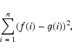
2.38 and 4.08 ![]() m and the absolute flux-values in this
wavelength range of the ISO-SWS spectrum, the angular diameter was
deduced. We therefore have minimised the residual sum of
squares
m and the absolute flux-values in this
wavelength range of the ISO-SWS spectrum, the angular diameter was
deduced. We therefore have minimised the residual sum of
squares
 |
The error bars on the
atmospheric parameters were estimated from 1. the intrinsic
uncertainty on the synthetic spectrum (i.e. the possibility to
distinguish different synthetic spectra at a specific resolution,
i.e. there should be a significant difference in ![]() -values)
which is thus dependent on both the resolving power of the
observation and the specific values of the fundamental parameters,
2. the uncertainty on the ISO-SWS spectrum which is directly
related to the S/N of the ISO-SWS observation, 3. the value
of the
-values)
which is thus dependent on both the resolving power of the
observation and the specific values of the fundamental parameters,
2. the uncertainty on the ISO-SWS spectrum which is directly
related to the S/N of the ISO-SWS observation, 3. the value
of the ![]() -parameters in the Kolmogorov-Smirnov test and 4. the still remaining discrepancies between observed and synthetic
spectra.
-parameters in the Kolmogorov-Smirnov test and 4. the still remaining discrepancies between observed and synthetic
spectra.
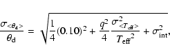
It should be noted that an error on the effective temperature
introduces an error on the angular diameter. The IR flux of the cool
giants does not follow the Rayleigh-Jeans law for a black-body, and we
can write
![]() .
Thus, with
.
Thus, with
![]() and
and
![]() ,
one obtains
,
one obtains
From the angular diameter and the parallax
measurements (mas) from Hipparcos (with an exception being
![]() Cen A, for which a more accurate parallax by Pourbaix et al. 1999, is
available), the stellar radius was
derived. This radius, together
with the gravity - determined from the ISO-SWS spectrum - then yielded
the gravity-inferred mass. From the radius and the effective
temperature, the stellar luminosity could be extracted.
Cen A, for which a more accurate parallax by Pourbaix et al. 1999, is
available), the stellar radius was
derived. This radius, together
with the gravity - determined from the ISO-SWS spectrum - then yielded
the gravity-inferred mass. From the radius and the effective
temperature, the stellar luminosity could be extracted.
This method of analysis could however not be applied to the warm stars of the sample. Absorption by atoms determines the spectrum of these stars. It turned out to be unfeasible to determine the effective temperature, gravity, microturbulence, metallicity and abundances of the chemical elements from the ISO-SWS spectra of these warm stars, due to
It seems important to cover a broad parameter space in order to be
able to distinguish between calibration problems and problems
related to the computation of a theoretical model and/or to the
generation of a synthetic spectrum. Therefore, stellar standard
candles spanning the spectral types A0-M8 were observed. The
observations were obtained in the context of two ISO-SWS
proposals. Some calibration data were also provided by the SIDT
(SWS Instrument Dedicated Team) in the framework of a
quick-feedback refining of the model SEDs used for the SWS
calibration. In total, full-resolution SWS scans of 20 standard
stars, covering the full A0-M8 spectral range were obtained.
Stars with an earlier spectral type were included in the proposals
of S. Price. An overview of the objects, observing dates and
integration times (
![]() )
can be found in Tables 1 and 2. Stars indicated by a "
)
can be found in Tables 1 and 2. Stars indicated by a "![]() '' are
stars which have been scrutinised more carefully than stars
indicated by a "
'' are
stars which have been scrutinised more carefully than stars
indicated by a "![]() ''. We first focused on
''. We first focused on ![]() Bootes
(K2 IIIp), because of its well-known stellar parameters and the
high quality of the ISO-SWS data for this object
(Decin et al. 1997). From then on, we have gone, step
by step, towards both higher and lower temperatures. Why the two
warmest stars in our sample (being Vega and Sirius) have been
considered, but have not been studied into all detail, will be
explained in Sect. 6.1. The other "
Bootes
(K2 IIIp), because of its well-known stellar parameters and the
high quality of the ISO-SWS data for this object
(Decin et al. 1997). From then on, we have gone, step
by step, towards both higher and lower temperatures. Why the two
warmest stars in our sample (being Vega and Sirius) have been
considered, but have not been studied into all detail, will be
explained in Sect. 6.1. The other "![]() ''-stars in Table 2 are stars cooler than an M2 giant - i.e. cooler than
''-stars in Table 2 are stars cooler than an M2 giant - i.e. cooler than
![]() 3500 K. Calibration problems with
3500 K. Calibration problems with ![]() Cru, variability
(Monnier et al. 1998), the possible presence of a
circumstellar envelope, stellar winds or a warm molecular envelope
above the photosphere (Tsuji et al. 1997) made the
use of hydrostatic models for these stars inappropriate and have
led to the decision to postpone the modelling of the coolest stars
in the sample.
Cru, variability
(Monnier et al. 1998), the possible presence of a
circumstellar envelope, stellar winds or a warm molecular envelope
above the photosphere (Tsuji et al. 1997) made the
use of hydrostatic models for these stars inappropriate and have
led to the decision to postpone the modelling of the coolest stars
in the sample.
| name | HD | HR | HIC | Spectral | AOT mode |
|
revo- |
| Type | (speed) | [sec] | lution | ||||
| 172167 | 7001 | 91262 | A0V | AOT01 (3) | 3462 | 178 | |
| Vega | AOT06 | 5642 | 650*1 | ||||
| AOT06 | 4354 | 678*2 | |||||
| 48915 | 2491 | 32349 | A1V | AOT01 (4) | 6538 | 689 | |
| Sirius | AOT01 (1) | 1140 | 868 | ||||
| 102647 | 4534 | 57632 | A3Vv | AOT01 (3) | 3462 | 189 | |
| Denebola | AOT01 (1) | 1096 | 040 | ||||
| Canopus | [0pt]45348 | [0pt]2326 | [0pt]30438 | [0pt]F0II | [0pt]AOT01 (4) | [0pt]6538 | [0pt]729 |
| 128620 | 5459 | 71683 | G2V | AOT01 (4) | 6538 | 607 | |
| AOT01 (1) | 1140 | 294 | |||||
| 180711 | 7310 | 94376 | G9III | AOT1 (4) | 6538 | 206 | |
| AOT01 (4) | 6528 | 072 | |||||
| 163588 | 6688 | 87585 | K2III | AOT01 (3) | 3454 | 314 | |
| AOT01 (1) | 1044 | 068 | |||||
| 124897 | 5340 | 69673 | K2IIIp | AOT01 (4) | 6538 | 452 | |
| Arcturus | AOT01 (4) | 6528 | 071 | ||||
| AOT01 (1) | 1140 | 275 | |||||
| AOT01 (1) | 1094 | 056 | |||||
| AOT06 | 3904 | 583*3 | |||||
| AOT06 | 4720 | 601*4 | |||||
| AOT06 | 4510 | 608*5 | |||||
| 211416 | 8502 | 110130 | K3III | AOT01 (4) | 6539 | 866 | |
| 131873 | 5563 | 72607 | K4III | AOT01 (4) | 6546 | 182 | |
| Kochab | AOT01 (2) | 1816 | 079 |
*1: 1A, 1B, 1D, 1E, 2A, 2B, 2C; *2: 1A, 1D, 1E, 2A;
*3: 1A, 1B, 1D, 2A, 2C; *4: 1A, 1B, 1D, 1E, 2A, 2B, 2C; *5:
1A, 1B, 1D, 1E, 2A, 2B, 2C.
| name | HD | HR | HIC | Spectral | AOT mode |
|
revo- |
| Type | (speed) | [sec] | lution | ||||
| 164058 | 6705 | 87833 | K5III | AOT01 (4) | 6538 | 377 | |
| Etamin | AOT01 (4) | 6542 | 040 | ||||
| AOT01 (2) | 1912 | 811 | |||||
| AOT01 (1) | 1140 | 496 | |||||
| AOT01 (1) | 1062 | 126 | |||||
| AOT06 | 4568 | 501*6 | |||||
| AOT06 | 5676 | 559*7 | |||||
| 29139 | 1457 | 21421 | K5III | AOT01(4) | 6538 | 636 | |
| Aldebaran | AOT06*8 | 3700 | 681 | ||||
| 149447 | 6166 | 81304 | K6III | AOT01(4) | 6538 | 847 | |
| 6860 | 337 | 5447 | M0III | AOT01 (4) | 6538 | 795 | |
| Mirach | AOT01 (3) | 3454 | 440 | ||||
| AOT01 (2) | 1912 | 423 | |||||
| 18884 | 911 | 14135 | M2III | AOT01 (4) | 6538 | 797 | |
| Menkar | AOT01 (4) | 6538 | 806 | ||||
| 217906 | 8775 | 113881 | M2.5III | AOT01(4) | 6538 | 551 | |
| Scheat | AOT01 (3) | 3454 | 206 | ||||
| AOT01 (1) | 1140 | 206 | |||||
| AOT01 (1) | 1096 | 056 | |||||
| 108903 | 4763 | 61084 | M4III | AOT01(4) | 6538 | 609 | |
| AOT01 (2) | 1912 | 258 | |||||
| AOT01 (2) | 1816 | 079 | |||||
| AOT06 | 5630 | 643*9 | |||||
| 214952 | 8636 | 112122 | M5III | AOT01 (3) | 3454 | 538 | |
| 148783 | 6146 | 80704 | M6III | AOT01 (4) | 6538 | 800 | |
| 194676 | 100935 | M7/8III | AOT01 (4) | 6538 | 872 |
*6: 1D, 1E, 2A, 2B, 2C; *7: 1A, 1B, 1D, 1E, 2A, 2B,
2C; *8: 1A, 1B, 1D, 1E, 2C; *9: 1A, 1B, 1D, 1E, 2A, 2B, 2C.
In order to reveal calibration problems, the ISO-SWS data have to
be reduced in a homogeneous way. For all the stars in our sample,
at least one AOT01 observation![]() (AOT = Astronomical Observation
Template; AOT01 = a single up-down scan for each aperture with
four possible scan speeds at degraded resolution) is available,
some stars have also been observed using the AOT06 mode (=long
up-down scan at full instrumental resolution). Since these AOT01
observations form a complete and consistent set, they were used as
the basis for the research. In order to check potential
calibration problems, the AOT06 data are used. The scanner speed
of the highest-quality AOT01 observations was 3 or 4, resulting in
a resolving power
(AOT = Astronomical Observation
Template; AOT01 = a single up-down scan for each aperture with
four possible scan speeds at degraded resolution) is available,
some stars have also been observed using the AOT06 mode (=long
up-down scan at full instrumental resolution). Since these AOT01
observations form a complete and consistent set, they were used as
the basis for the research. In order to check potential
calibration problems, the AOT06 data are used. The scanner speed
of the highest-quality AOT01 observations was 3 or 4, resulting in
a resolving power ![]() 870 or
870 or ![]() 1500, respectively
(Leech et al. 2002). The appropriate resolving power of each
sub-band was taken to be the most conservative theoretical
resolving power as determined by Lorente in Leech et al. (2002),
with the exception being band 1A for which this value has been
changed from 1500 to 1300, as will be discussed in Sect. 6.2.
1500, respectively
(Leech et al. 2002). The appropriate resolving power of each
sub-band was taken to be the most conservative theoretical
resolving power as determined by Lorente in Leech et al. (2002),
with the exception being band 1A for which this value has been
changed from 1500 to 1300, as will be discussed in Sect. 6.2.
The ISO-SWS data were processed to a calibrated spectrum by using the same procedure as described in Paper I using the calibration files available in OLP6.0.
The band 2 (Si:Ga) detectors used in SWS "remember'' their previous illumination history. Going from low to high illumination, or vice versa, results in detectors asymptotically reaching their new output value. These are referred to as memory effects or transients. For sources with fluxes greater than about 100 Jy, memory effects cause the up and down scans in the SPD (=Standard Processed Data) to differ in response by up to 20% in band 2. Since an adapted version of the Fouks-Schubert model to correct for these memory effects in band 2 was still in development (Leech et al. 2002), this method could not be applied during our reduction procedure. Instead, we have used the down-scan data of our observation as a reference to do a correction of the flux level of the first scan (up-scan). This is justified since the memory effects appear to be less severe in the down-scan measurements, suggesting a more stabilised response to the flux level for the down-scan data.
Also the band 2 dark current subtraction is closely tied to the band 2 memory effect correction. The memory effect for Si:Ga detectors as described by the Fouks-Schubert model is an additive effect. As such, its proper correction will take place during the dark current subtraction. Since this correction tool was still not available, all dark currents were checked individually. When a dark current was corrupted too much by memory effects, its value was replaced by the value of a preceding or following dark-current not being affected. In this way, a small error can occur, which is, however, negligible due to the high flux level of our stellar sources.
| 1A | 1B | 1D | 1E | 2A | 2B | 2C | rev. | dy | dz | |
|
|
1300 | 1200 | 1500 | 1000 | 1200 | 800 | 800 | |||
|
|
2.38 | 2.60 | 3.02 | 3.52 | 4.08 | 5.30 | 7.00 | |||
|
|
2.60 | 3.02 | 3.52 | 4.08 | 5.30 | 7.00 | 12.00 | |||
| 1.06 | 1.06 | 1.00 | 1.00 | 1.00 | 0.97 | +12Jy | 178 | -0.608 | -1.179 | |
| 1.00 | 1.00 | 1.00 | 0.995 | 1.12 | 1.23 | 1.00 | 689 | 0.034 | 0.003 | |
| 0.99 | 0.99 | 1.00 | 1.00 | 1.16 | 1.27 | +3.5Jy | 189 | 0.478 | 0.556 | |
| 0.97 | 0.98 | 1.00 | 1.00 | 0.98 | 1.10 | 0.91 | 729 | 0.024 | 0.072 | |
| 1.01 | 1.02 | 1.00 | 1.01 | 0.985 | 1.06 | 0.91 | 607 | 0.000 | 0.000 | |
| 0.97 | 0.98 | 1.00 | 1.015 | 1.03 | 1.02 | 1.10 | 206 | -0.422 | 1.480 | |
| 0.99 | 0.99 | 1.00 | 0.99 | 1.12 | 1.15 | 1.05 | 314 | 1.286 | -0.282 | |
| 0.995 | 1.01 | 1.00 | 1.005 | 0.95 | 1.05 | 1.00 | 452 | 0.000 | 0.000 | |
| 1.005 | 1.02 | 1.00 | 1.01 | 1.05 | 1.00 | 1.00 | 866 | 0.000 | 0.000 | |
| 1.00 | 1.015 | 1.00 | 1.01 | 0.91 | 0.885 | 1.00 | 182 | -1.062 | 0.045 | |
| 0.995 | 1.005 | 1.00 | 1.005 | 0.935 | 0.98 | 0.91 | 377 | -0.304 | 0.181 | |
| 1.00 | 1.01 | 1.00 | 1.00 | 1.00 | 1.045 | 1.00 | 636 | 0.000 | 0.000 | |
| H Sco | 1.00 | 1.015 | 1.00 | 1.00 | 1.13 | 1.05 | 1.15 | 847 | 0.000 | 0.000 |
| 1.00 | 1.00 | 1.00 | 1.005 | 1.00 | 1.10 | 0.95 | 795 | 0.000 | 0.000 | |
| 0.985 | 1.00 | 1.00 | 1.01 | 0.935 | 1.03 | 0.91 | 797 | 0.000 | 0.000 | |
| 1.00 | 1.015 | 1.00 | 1.005 | 0.935 | 1.03 | 0.935 | 551 | 0.017 | 0.095 |
Since the different sub-band spectra can show jumps in flux at the
band-edges, several sub-bands had to be multiplied by a small
factor to construct a smooth spectrum. Three causes for the
observed shift factors between different sub-bands of an
observation and between different observations of a given stellar
source can be reported: 1. pointing errors, 2. problems with the
RSRF correction, and 3. a problematic dark current subtraction,
from which the pointing errors are believed to have the largest
impact. The pointing errors as well as the RSRF correction causes
a decrease in flux by a gain factor, while the dark current
subtraction can lower the flux level by an offset. As the effects
of the pointing errors are estimated to have the biggest effect,
and since the stars in our sample have a high flux level so that
the dark current subtraction only plays a marginal role, the
individual sub-bands were multiplied with a factor - rather than
shifted with an offset - in order to obtain a smooth spectrum.
These factors (see Table 3) were determined by using
the overlap regions of the different sub-bands and by studying the
other SWS observations. The band-1D data were taken as reference
data, due to the absence of strong molecular absorption in
this wavelength range which may cause a higher standard deviation
in the bins obtained when rebinning the oversampled spectrum, and
- most importantly - due to the low systematic errors in this
band, caused by e.g. errors in the curve of the RSRF, detector
noise, uncertainties in the conversion factors from ![]() V/s to
Jy, ... (Leech et al. 2002). Using the total absolute uncertainty
values - which have accumulated factors from each of the
calibration steps plus estimated contributions from processes
which were unprobed or uncorrected - as given in Table 5.3 in
Leech et al. (2002), the estimated 1
V/s to
Jy, ... (Leech et al. 2002). Using the total absolute uncertainty
values - which have accumulated factors from each of the
calibration steps plus estimated contributions from processes
which were unprobed or uncorrected - as given in Table 5.3 in
Leech et al. (2002), the estimated 1 ![]() uncertainty on these
factors is 10%. As is clearly visible from Table 3, these factors do not show any trend with spectral
type or flux-level. This is displayed in Fig. 1, where the band-border ratios between 1A-1B, 1B-1D
and 1D-1E are plotted in function of the flux at 2.60, 3.02 and
3.52
uncertainty on these
factors is 10%. As is clearly visible from Table 3, these factors do not show any trend with spectral
type or flux-level. This is displayed in Fig. 1, where the band-border ratios between 1A-1B, 1B-1D
and 1D-1E are plotted in function of the flux at 2.60, 3.02 and
3.52 ![]() m respectively. For this plot, all the observations of
the cool stars in our sample, discussed in the Appendix of
Paper IV of this series, are used. In band 1, the band-border
ratios of 1A-1B and 1D-1E are from bands within the same aperture.
Going from band 1B to band 1D, the aperture changes. Satellite
mispointings can have a pernicious impact on this band-border
ratio: the mean deviation of the band-border ratios w.r.t. 1 is
significantly larger for 1B-1D (=0.015) than for 1A-1B and 1D-1E
(being respectively 0.009 and 0.005). Due to the problems with
memory effects in band 2 (4.08-12
m respectively. For this plot, all the observations of
the cool stars in our sample, discussed in the Appendix of
Paper IV of this series, are used. In band 1, the band-border
ratios of 1A-1B and 1D-1E are from bands within the same aperture.
Going from band 1B to band 1D, the aperture changes. Satellite
mispointings can have a pernicious impact on this band-border
ratio: the mean deviation of the band-border ratios w.r.t. 1 is
significantly larger for 1B-1D (=0.015) than for 1A-1B and 1D-1E
(being respectively 0.009 and 0.005). Due to the problems with
memory effects in band 2 (4.08-12 ![]() m), the factors of each
sub-band of band 2 were determined by use of the corresponding
spectral data of Cohen (Cohen et al. 1992, 1995, 1996;
Witteborn et al. 1999): for Vega and Sirius Cohen has
constructed a calibrated model spectrum; a composite spectrum
(i.e. various observed spectra have been spliced to each other
using photometric data) is available for
m), the factors of each
sub-band of band 2 were determined by use of the corresponding
spectral data of Cohen (Cohen et al. 1992, 1995, 1996;
Witteborn et al. 1999): for Vega and Sirius Cohen has
constructed a calibrated model spectrum; a composite spectrum
(i.e. various observed spectra have been spliced to each other
using photometric data) is available for ![]() Cen A,
Cen A, ![]() Boo,
Boo, ![]() Dra,
Dra, ![]() Tau,
Tau, ![]() And,
And, ![]() Cet, and
Cet, and
![]() Peg; a template spectrum (i.e. a spectrum made by using
photometric data of the star itself and the shape of a "template''
star) is built for
Peg; a template spectrum (i.e. a spectrum made by using
photometric data of the star itself and the shape of a "template''
star) is built for ![]() Dra (template:
Dra (template: ![]() Gem: K0 III),
Gem: K0 III),
![]() Dra (template:
Dra (template: ![]() Boo: K2 IIIp),
Boo: K2 IIIp), ![]() Tuc
(template:
Tuc
(template: ![]() Hya: K3 II-III) and H Sco (template:
Hya: K3 II-III) and H Sco (template: ![]() Tau: K5 III). When no template was available (for
Tau: K5 III). When no template was available (for ![]() Leo,
Leo, ![]() Car and
Car and ![]() UMi), the synthetic spectrum
showing the best agreement with the band-1 data was used as
reference. This does not imply that we are trapped in a circular
argument, since the stellar parameters for the synthetic spectrum
were determined from the band-1 data only. Moreover, the
maximum difference in the correction factors for band 2 obtained
when using the synthetic spectra instead of a Cohen template for
the 13 stars common in the sample is 7%, which is well within
the photometric absolute flux uncertainties claimed by
Leech et al. (2002). Note that all shift factors are in within the
AOT01 band border ratios as derived in Figs. 5.33 and 5.34
in Leech et al. (2002). Using the overlap regions in band 2 can
have quite a big effect on the final composed spectrum: focussing
on
UMi), the synthetic spectrum
showing the best agreement with the band-1 data was used as
reference. This does not imply that we are trapped in a circular
argument, since the stellar parameters for the synthetic spectrum
were determined from the band-1 data only. Moreover, the
maximum difference in the correction factors for band 2 obtained
when using the synthetic spectra instead of a Cohen template for
the 13 stars common in the sample is 7%, which is well within
the photometric absolute flux uncertainties claimed by
Leech et al. (2002). Note that all shift factors are in within the
AOT01 band border ratios as derived in Figs. 5.33 and 5.34
in Leech et al. (2002). Using the overlap regions in band 2 can
have quite a big effect on the final composed spectrum: focussing
on ![]() UMi, we note that by using these overlap regions band
2A (and consequently bands 2B and 2C) should be shifted downwards
by a factor 1.04; in order then to match the shifted band 2B and
band 2C, band 2C should be once more shifted downwards by a factor
1.12. In general, the error in the absolute flux could increase to
UMi, we note that by using these overlap regions band
2A (and consequently bands 2B and 2C) should be shifted downwards
by a factor 1.04; in order then to match the shifted band 2B and
band 2C, band 2C should be once more shifted downwards by a factor
1.12. In general, the error in the absolute flux could increase to
![]() 20% at the end of band 2C when this method would be
used.
20% at the end of band 2C when this method would be
used.
For a more elaborate discussion on the SWS error budget, we would like to refer to Leech et al. (2002).
![\begin{figure}
\par\includegraphics[width=8.8cm,clip]{h3317f1_bw.ps}
\end{figure}](/articles/aa/full/2003/11/aah3317/img52.gif) |
Figure 1: Flux ratios between the different sub-bands of band 1 at the wavelengths of overlap. The mean deviation w.r.t. 1 is given for the different band borders at the right corner of the figure. |
| Open with DEXTER | |
To test our findings - indicating either a calibration problem or a
theoretical modelling problem - with data taken with an independent
instrument, a high-resolution observation of both one warm
and one cool star were included. The
high-resolution Fourier Transform Spectrometer (FTS) spectrum of
![]() Boo (Hinkle et al. 1995b) and the Atmospheric Trace
Molecule Spectroscopy (ATMOS) spectrum of the
Sun (Farmer & Norton 1989; Geller 1992) are used as external
control to the process.
Boo (Hinkle et al. 1995b) and the Atmospheric Trace
Molecule Spectroscopy (ATMOS) spectrum of the
Sun (Farmer & Norton 1989; Geller 1992) are used as external
control to the process.
The Arcturus observations were obtained with the FTS at the Kitt
Peak (KP) 4 m Mayall telescope mainly in 1993 and 1994 and are described in
Hinkle et al. (1995a); Hinkle et al. (1995b). The entirety of the 1 to
5 ![]() m Arcturus
spectrum detectable from the ground was observed twice at opposite
heliocentric velocities, allowing the removal of many telluric
lines. We refer to these two
spectra as the winter and summer observations. The data were obtained
at a resolving power (
m Arcturus
spectrum detectable from the ground was observed twice at opposite
heliocentric velocities, allowing the removal of many telluric
lines. We refer to these two
spectra as the winter and summer observations. The data were obtained
at a resolving power (![]() /
/
![]() )
near 100 000.
Spectra of the Earth's atmosphere, derived from high resolution solar
spectra, have been ratioed to the Arcturus spectra to largely remove the
telluric lines. Most telluric lines less than 30% deep are cleanly
removed but as the optical depth of the telluric lines increases more
information is lost and lines over 50% deep can not be removed. Gaps
in the plots appear at these spectral regions. A typical example of
the Arcturus spectra is shown in Fig. 16 on page
)
near 100 000.
Spectra of the Earth's atmosphere, derived from high resolution solar
spectra, have been ratioed to the Arcturus spectra to largely remove the
telluric lines. Most telluric lines less than 30% deep are cleanly
removed but as the optical depth of the telluric lines increases more
information is lost and lines over 50% deep can not be removed. Gaps
in the plots appear at these spectral regions. A typical example of
the Arcturus spectra is shown in Fig. 16 on page ![]() . In the upper panel of Fig. 16, some CO lines of the first overtone are plotted. In the lower
panel of Fig. 16, one can clearly distinguish atomic and OH lines.
. In the upper panel of Fig. 16, some CO lines of the first overtone are plotted. In the lower
panel of Fig. 16, one can clearly distinguish atomic and OH lines.
During the period from November 3 to November 14, 1994, the Atmospheric Trace Molecule Spectroscopy (ATMOS) experiment operated as part of the ATLAS-3 payload of the shuttle Atlantis (Gunson et al. 1996). The principal purpose of this experiment was to study the distribution of the atmosphere's trace molecular components. The instrument, a modified Michelson interferometer, covering the frequency range from 625 to 4800 cm-1 at a spectral resolution of 0.01 cm-1, also recorded high-resolution infrared spectra of the Sun. A small part of the intensity spectrum is shown in Fig. 2. The Holweger-Müller model (Holweger & Müller 1974) was used as input for the computation of the synthetic spectrum of the Sun. A microturbulent velocity of 1 km s-1 was assumed.
![\begin{figure}
\par\includegraphics[angle=90,width=8.8cm,clip]{h3317f2_bw.ps}
\end{figure}](/articles/aa/full/2003/11/aah3317/img56.gif) |
Figure 2:
FTS-ATMOS intensity spectrum of the Sun (black)
at a resolving power
|
| Open with DEXTER | |
In the case of ![]() Boo, a high-resolution synthetic spectrum was first
generated with the stellar parameters of
Kjærgaard et al. (1982) as input parameters (
Boo, a high-resolution synthetic spectrum was first
generated with the stellar parameters of
Kjærgaard et al. (1982) as input parameters (
![]() K,
K,
![]() ,
[Fe/H] = -0.50,
,
[Fe/H] = -0.50,
![]() (C) = 7.89,
(C) = 7.89,
![]() (N) = 7.61,
(N) = 7.61,
![]() (O) = 8.68). For the
microturbulence
(O) = 8.68). For the
microturbulence
![]() a
velocity of 1.7 km s-1 was assumed as being the mean for red giants
(Gustafsson et al. 1974). Since both
Mäckle et al. (1975) and Bell et al. (1985)
found a Si and Mg abundance depleted with respect to the solar values,
a
velocity of 1.7 km s-1 was assumed as being the mean for red giants
(Gustafsson et al. 1974). Since both
Mäckle et al. (1975) and Bell et al. (1985)
found a Si and Mg abundance depleted with respect to the solar values,
![]() (Mg) was taken to be 7.33 and
(Mg) was taken to be 7.33 and
![]() (Si) to be
7.20. For
the anisotropic macroturbulence
(Si) to be
7.20. For
the anisotropic macroturbulence
![]() ,
a radial-tangential
profile was assumed (Gray 1975) with FWHM of 3 km s-1.
This synthetic spectrum was then convolved with the beam-profile
function (i.e. a sinc-function). Both observed FTS-KP and synthetic
spectrum were
rebinned to a resolving power of 60 000, since the resolving power of
the FTS-KP was not constant over the whole wavelength range.
Using this set of input-parameters, the high-excitation CO (
,
a radial-tangential
profile was assumed (Gray 1975) with FWHM of 3 km s-1.
This synthetic spectrum was then convolved with the beam-profile
function (i.e. a sinc-function). Both observed FTS-KP and synthetic
spectrum were
rebinned to a resolving power of 60 000, since the resolving power of
the FTS-KP was not constant over the whole wavelength range.
Using this set of input-parameters, the high-excitation CO (
![]() and
and
![]() )
and SiO (
)
and SiO (
![]() )
lines were predicted as being
too weak. This was confirmed from both the FTS-KP and the
ISO-SWS spectrum. Especially from the ISO-SWS spectrum - and more
specifically from the slope in bands 1B and 1D - it became clear that
the gravity should be lowered. Using then
the FTS-KP-spectra, the input parameters were
improved until an optimal fit was obtained (see Fig. 16 on
page
)
lines were predicted as being
too weak. This was confirmed from both the FTS-KP and the
ISO-SWS spectrum. Especially from the ISO-SWS spectrum - and more
specifically from the slope in bands 1B and 1D - it became clear that
the gravity should be lowered. Using then
the FTS-KP-spectra, the input parameters were
improved until an optimal fit was obtained (see Fig. 16 on
page ![]() ). This
resulted in the
following parameters:
). This
resulted in the
following parameters:
![]() K,
K,
![]() ,
[Fe/H] = -0.50,
,
[Fe/H] = -0.50,
![]() km s-1,
km s-1,
![]() ,
,
![]() (C) = 7.96,
(C) = 7.96,
![]() (N) = 7.61,
(N) = 7.61,
![]() (O)
= 8.68,
(O)
= 8.68,
![]() (Mg) = 7.33 and
(Mg) = 7.33 and
![]() (Si) = 7.20.
(Si) = 7.20.
Discrepancies appearing from the confrontation of the synthetic spectrum with both the FTS-KP and the ISO-SWS spectra, may be clearly attributed to problems in constructing the model or generating the synthetic spectrum. Other discrepancies in the ISO-SWS versus synthetic spectrum are the ones caused by calibration problems.
For the warm stars in the sample, an analogous
comparison was performed with the help of the FTS-ATMOS intensity
spectrum of the Sun. Discrepancies between the ISO-SWS and
synthetic spectra of ![]() Cen A (G2V) were compared with the
discrepancies found in the comparison between the FTS-ATMOS spectrum
of the Sun and its synthetic spectrum (Fig. 2).
Cen A (G2V) were compared with the
discrepancies found in the comparison between the FTS-ATMOS spectrum
of the Sun and its synthetic spectrum (Fig. 2).
Inspecting Figs. 2 and 16, some discrepancies become immediately visible, e.g. the CO 2-0 and 3-1 are predicted too weak in both figures. The reason for this and other discrepancies will be explained in the next section.
Computing synthetic spectra is one step, distilling useful information from it is a second - and far more difficult - one. Fundamental stellar parameters for this sample of bright stars are a first direct result which can be deduced from this comparison between ISO-SWS data and synthetic spectra. In Papers III and IV of this series, these parameters will be discussed and confronted with other published stellar parameters.
![\begin{figure}
\par\includegraphics[angle=90,width=8.8cm,clip]{h3317f3_col.ps}
\end{figure}](/articles/aa/full/2003/11/aah3317/img70.gif) |
Figure 3:
Comparison between the ISO-SWS data of
|
| Open with DEXTER | |
![\begin{figure}
\par\includegraphics[width=8.8cm,clip]{aah3317new/h3317f4_col.eps}
\end{figure}](/articles/aa/full/2003/11/aah3317/img76.gif) |
Figure 4:
Comparison between band 1 and band 2 of
the ISO-SWS data of |
| Open with DEXTER | |
A typical example of both a warm and cool star is given in
Figs. 3 and 4 respectively. Different types of
discrepancies do emerge. The size of the discrepancies between
ISO-SWS observations and theoretical predictions varies a lot.
Both for the warm and for the cool stars we see a general
good agreement in shape between the ISO-SWS and theoretical data in
band 1, with however (local) error peaks up to ![]() 8%. An exception
is
8%. An exception
is ![]() Peg for which the shape is wrong by
Peg for which the shape is wrong by ![]() 6% and local
error peaks may go up to
6% and local
error peaks may go up to ![]() 15%. The agreement between
observational and synthetic data is worse in band 2: a general
mismatch by up to
15%. The agreement between
observational and synthetic data is worse in band 2: a general
mismatch by up to ![]() 15% may occur.
15% may occur.
By scrutinising carefully the various discrepancies between the ISO-SWS data and the synthetic spectra of the standard stars in our sample, the origin of the different discrepancies was elucidated. First of all, a description on the general trends in discrepancies for the warm stars will be made, after which the cool stars will be discussed.
![\begin{figure}
\par\includegraphics[angle=90,width=8.8cm,clip]{h3317f5_bw.ps}
\end{figure}](/articles/aa/full/2003/11/aah3317/img77.gif) |
Figure 5:
In panel a) the high-resolution FTS-ATMOS
spectrum of the Sun is compared with its synthetic spectrum based
on the Holweger-Müller model (1974) and computed by using the
atomic line list of Hirata & Horaguchi (1995). Panel b) shows the same
comparison as panel a), but now at a resolving power of 1000 for
the wavelength range going from 3.52-4.08 |
| Open with DEXTER | |
For Fig. 5, the atomic line list of Hirata & Horaguchi (1995) was used to generate the synthetic spectrum. This line list has as starting files the compilation by Kurucz & Peytremann (1975) and Kurucz (1989) who lists the semi-empirical gf-values for many ions. Energy levels were adopted from recent compilations (Sugar & Corliss 1985) or individual works. The line list of Kelly (1983) was merged into the file. The gf-values are taken from several compilations (e.g. Fuhr et al. 1988a, 1988b; Reader et al. 1980; Wiese et al. 1966, 1969; Morton 1991, 1992). Published results of the Opacity Project (Seaton 1995) were also included. Comparing the atomic line list of Hirata & Horaguchi (1995) with the identifications as given by Geller (1992) made clear that quite some lines are misidentified or not included in the IR atomic line list of Hirata & Horaguchi (1995).
The usage of VALD (Vienna Atomic Line
Database: Piskunov et al. 1995;
Ryabchikova et al. 1997;
Kupka et al. 1999)![]() and the line list of van Hoof (1998)
did not solve the problem.
Obviously, the oscillator strengths of the atomic lines in the
infrared are not known sufficiently well.
and the line list of van Hoof (1998)
did not solve the problem.
Obviously, the oscillator strengths of the atomic lines in the
infrared are not known sufficiently well.
In order to test this hypothesis, Sauval (2002, priv. comm.) has constructed a new atomic line list by deducing new oscillator strengths from the high-resolution ATMOS spectra of the Sun (625-4800 cm-1). A preliminary comparison using this new linelist is given in Fig. 6 (which should be compared with Fig. 5). The contents, nature, limitations, uncertainties, ... of this new line list will be discussed in a forthcoming paper. But it is already obvious from a confrontation between Figs. 5 and 6 that these new oscillator strengths from Sauval are more accurate.
![\begin{figure}
\par\includegraphics[angle=90,width=8.8cm,clip]{h3317f6_bw.ps}
\end{figure}](/articles/aa/full/2003/11/aah3317/img78.gif) |
Figure 6:
In panel a) the high-resolution ATMOS
spectrum of the Sun is compared with its synthetic spectrum based
on the Holweger-Müller model (1974) and computed by using the
atomic line list of Sauval (2002, priv. comm.). Panel b) shows the same
comparison as panel a), but now at a resolving power of 1000 for
the wavelength range going from 3.52-4.08 |
| Open with DEXTER | |
It is plausible that the same reason, i.e. wrong and missing oscillator strengths of atomic lines in the infrared, together with noise, is the origin of the observed discrepancies between the ISO-SWS and synthetic spectra for the other warm stars in the sample, because
![\begin{figure}
\par\includegraphics[angle=90,width=8.8cm,clip]{h3317f7_bw.ps}
\end{figure}](/articles/aa/full/2003/11/aah3317/img79.gif) |
Figure 7:
FTS-ATMOS intensity spectrum of the Sun
(black) at a resolving power
|
| Open with DEXTER | |
![\begin{figure}
\par\includegraphics[angle=90,width=8.8cm,clip]{h3317f8_bw.ps}
\end{figure}](/articles/aa/full/2003/11/aah3317/img81.gif) |
Figure 8:
Comparison between the observed ISO-SWS
spectrum of |
| Open with DEXTER | |
![\begin{figure}
\par\includegraphics[angle=90,width=8.8cm,clip]{h3317f9_bw.ps}
\end{figure}](/articles/aa/full/2003/11/aah3317/img83.gif) |
Figure 9:
Band 1A of Vega (A0 V), |
| Open with DEXTER | |
![\begin{figure}
\par\includegraphics[angle=90,width=8.8cm,clip]{h3317f10_col.ps}
\end{figure}](/articles/aa/full/2003/11/aah3317/img85.gif) |
Figure 10:
Band 2 for Sirius (A1 V) and |
| Open with DEXTER | |
![\begin{figure}
\par\includegraphics[angle=90,width=8.8cm,clip]{h3317f11_col.ps}
\end{figure}](/articles/aa/full/2003/11/aah3317/img88.gif) |
Figure 11:
Comparison between the ISO-SWS observation and the
synthetic spectrum of |
| Open with DEXTER | |
In these oxygen-rich stars, the CO lines are a direct measure of the C abundance. From the present spectra, this carbon abundance can be estimated in two ways:
A first step towards solving this problem was the use of the
high-resolution FTS-KP spectrum of ![]() Boo (see Sect. 5). As was explained in Sect. 5 a
high-resolution synthetic spectrum was generated for
Boo (see Sect. 5). As was explained in Sect. 5 a
high-resolution synthetic spectrum was generated for ![]() Boo
and rebinned to a resolution of 60 000. The agreement between the
observed FTS-KP and synthetic spectrum is extremely good! One
example was already shown in Fig. 16, another one is
depicted in Fig. 17 on page
Boo
and rebinned to a resolution of 60 000. The agreement between the
observed FTS-KP and synthetic spectrum is extremely good! One
example was already shown in Fig. 16, another one is
depicted in Fig. 17 on page ![]() . In this
latter figure, the problematic subtraction of the atmospheric
contribution causes the spurious features around 2.46700
. In this
latter figure, the problematic subtraction of the atmospheric
contribution causes the spurious features around 2.46700 ![]() m for the summer FTS-KP spectrum and around 2.46735
m for the summer FTS-KP spectrum and around 2.46735 ![]() m for the
winter FTS-KP spectrum
m for the
winter FTS-KP spectrum![]() . When scrutinising carefully the
first-overtone CO lines in the FTS-KP spectrum, it is obvious that
all the 12CO 2-0 lines, and almost all the 12CO 3-1
lines, are predicted as too weak (by 1-2%) and not as
too strong as was suggested in previous paragraph from the
comparison between ISO-SWS and synthetic spectra! Also the
fundamental CO lines are predicted as being a few percent too
weak. For a better judgement of the KP-SWS-synthetic
correspondence, the FTS-KP spectrum was rebinned to the ISO
resolving power. This was not so straightforward due to the
presence of the spurious features originating from the problematic
subtraction of the atmospheric contribution. In order to conserve
the flux, these spurious features were replaced by the flux value
of the synthetic spectrum. This adaptation is acceptable for the
following reasons:
. When scrutinising carefully the
first-overtone CO lines in the FTS-KP spectrum, it is obvious that
all the 12CO 2-0 lines, and almost all the 12CO 3-1
lines, are predicted as too weak (by 1-2%) and not as
too strong as was suggested in previous paragraph from the
comparison between ISO-SWS and synthetic spectra! Also the
fundamental CO lines are predicted as being a few percent too
weak. For a better judgement of the KP-SWS-synthetic
correspondence, the FTS-KP spectrum was rebinned to the ISO
resolving power. This was not so straightforward due to the
presence of the spurious features originating from the problematic
subtraction of the atmospheric contribution. In order to conserve
the flux, these spurious features were replaced by the flux value
of the synthetic spectrum. This adaptation is acceptable for the
following reasons:
Figure 18 on page ![]() shows the
comparison between the ISO-SWS,
the FTS-KP and the synthetic spectrum for
shows the
comparison between the ISO-SWS,
the FTS-KP and the synthetic spectrum for ![]() Boo at a resolving
power of 1500. It is clear that the differences between the
strength of the CO features in the ISO-SWS and FTS-KP spectrum are
significant. This is a strong indication for problems in the
calibration process. The question now arises where this
calibration problem originates from.
Boo at a resolving
power of 1500. It is clear that the differences between the
strength of the CO features in the ISO-SWS and FTS-KP spectrum are
significant. This is a strong indication for problems in the
calibration process. The question now arises where this
calibration problem originates from.
Firstly, it has to be noted that the flux values are unreliable in the
wavelength region from 2.38 to 2.40 ![]() m due to problems with the
RSRF of band 1A; main features here include the CO 2-0 P18 and
the CO 2-0 P21 lines.
m due to problems with the
RSRF of band 1A; main features here include the CO 2-0 P18 and
the CO 2-0 P21 lines.
Secondly, no correlation is found with the local minima and maxima in the RSRF of band 1A.
![\begin{figure}
\par\includegraphics[angle=90,width=8.8cm,clip]{h3317f12_col.ps}
\end{figure}](/articles/aa/full/2003/11/aah3317/img89.gif) |
Figure 12:
Comparison between the AOT06 observation
(revolution 538, black) and the AOT01 speed-4 observation (grey) of
|
| Open with DEXTER | |
Defining the spectral resolution and instrumental profile for the ISO-SWS
grating spectrometers, is not straightforward (Lorente 1998;
Lutz et al. 1999). Only for an AOT02 observation has the instrumental profile now been
derived quite accurately (Lutz et al. 1999). The AOT01 mode introduces an
additional smoothing which, due to the intricacies of SWS-data acquisition, is
different from a simple boxcar smooth. The simulation of SWS-AOT01 scans gives
non-gaussian profiles, as can be seen in Fig. 6 by Lorente (1998).
Nevertheless, the theoretical profile of a speed-4 observation
approximates a gaussian profile very closely. Therefore, since the instrumental
profile of an AOT01 is still not exactly known, the synthetic data were
convolved with a gaussian with
![]() /resolution. This incorrect
gaussian instrumental profile introduces an error which will be most visible on
the strongest lines.
/resolution. This incorrect
gaussian instrumental profile introduces an error which will be most visible on
the strongest lines.
![\begin{figure}
\par\includegraphics[angle=90,width=8.8cm,clip]{h3317f13_col.ps}
\end{figure}](/articles/aa/full/2003/11/aah3317/img91.gif) |
Figure 13:
Top: Comparison between the
AOT01 speed-4 observation of |
| Open with DEXTER | |
Only for ![]() Dra an AOT06 observation, scanning this
wavelength range, was available in the ISO data-archive. The
comparison between the AOT01 speed-4 and AOT06 observation, both
rebinned to a resolving power of 1500, is an indication that the
resolving power of an AOT01 speed-4 observation in band 1A is lower
than 1500 (Fig. 12). The theoretical resolving power for an
AOT01 speed-4 observation in band 1A is
Dra an AOT06 observation, scanning this
wavelength range, was available in the ISO data-archive. The
comparison between the AOT01 speed-4 and AOT06 observation, both
rebinned to a resolving power of 1500, is an indication that the
resolving power of an AOT01 speed-4 observation in band 1A is lower
than 1500 (Fig. 12). The theoretical resolving power for an
AOT01 speed-4 observation in band 1A is ![]() 1500. Figure 5 in
Lorente (1998) shows, however, a large deviation from this value,
attributed to the fainter continuum of the source used for
measuring the instrumental profile and the less accurate fitting in
this band. The use of a resolving power of 1300 - instead of the
theoretical resolving power of 1500 - for band 1A yields a) almost
no difference from the AOT01 SWS data at a resolving power of 1500 and b) a
better match between the SWS and synthetic data for the
strongest CO features (Fig. 13). This observational resolving power of 1300 is also
in good agreement with the observational value given by Lorente (1998) in
her Fig. 5.
1500. Figure 5 in
Lorente (1998) shows, however, a large deviation from this value,
attributed to the fainter continuum of the source used for
measuring the instrumental profile and the less accurate fitting in
this band. The use of a resolving power of 1300 - instead of the
theoretical resolving power of 1500 - for band 1A yields a) almost
no difference from the AOT01 SWS data at a resolving power of 1500 and b) a
better match between the SWS and synthetic data for the
strongest CO features (Fig. 13). This observational resolving power of 1300 is also
in good agreement with the observational value given by Lorente (1998) in
her Fig. 5.
The incorrect use of a Gaussian instrumental profile, together with too high a - theoretical - resolving power of 1500 form the origin of the discrepancy seen for the strongest CO features. Therefore, the resolving power of band 1A was taken to be 1300 instead of 1500. Part of the other discrepancies seen in band 1A may be explained by problems with 1. the accuracy of the oscillator strengths of atomic transitions in the near-IR (see point 1. in this section) or 2. the RSRF in the beginning of band 1A (see point 5. in previous section).
![\begin{figure}
\par\includegraphics[angle=90,width=8.8cm,clip]{h3317f14_col.ps}
\end{figure}](/articles/aa/full/2003/11/aah3317/img93.gif) |
Figure 14:
Summer and winter FTS-KP
spectra of |
| Open with DEXTER | |
The results of this detailed comparison between observed ISO-SWS data and synthetic spectra have an impact both on the calibration of the ISO-SWS data and on the theoretical description of stellar atmospheres.
From the calibration point of view, a first conclusion is reached
that the broad-band shape of the relative spectral response
function is at the moment already quite accurate, although some
improvements can be made at the beginning of band 1A (see Fig. 15) and band 2. Also, a fringe pattern is
recognised at the end of band 1D. Inaccuracies in the adopted
instrumental profile used to convolve the synthetic spectra with,
together with too high a resolving power, may cause the strongest
CO
![]() band heads in the observed ISO-SWS spectrum to
be weaker than the predicted line strength.
band heads in the observed ISO-SWS spectrum to
be weaker than the predicted line strength.
![\begin{figure}
\par\includegraphics[angle=90,width=8.8cm,clip]{h3317f15_bw.ps}
\end{figure}](/articles/aa/full/2003/11/aah3317/img94.gif) |
Figure 15:
The observed ISO-SWS spectra of some
stars with different spectral types are divided by their synthetic
spectrum calculated by using the atomic line list of
Hirata & Horaguchi (1995). The ratio is rebinned to a resolving power of
250. Only
at the beginning of band 1A the same trend is visible in all stars,
indicating that the broad-band shape of the relative
spectral-response functions is already quite accurately known for
the different sub-bands of band 1, with the only exception being
at the beginning of band 1A. The feature arising around 3.85 |
| Open with DEXTER | |
![\begin{figure}
\par\includegraphics[angle=90,width=8.5cm,clip]{h3317f16_col.eps}
\end{figure}](/articles/aa/full/2003/11/aah3317/img95.gif) |
Figure 16:
Summer (red) and winter (green) FTS-KP spectrum of
|
| Open with DEXTER | |
![\begin{figure}
\par\includegraphics[angle=90,width=8.5cm,clip]{h3317f17_col.eps}
\end{figure}](/articles/aa/full/2003/11/aah3317/img96.gif) |
Figure 17:
Summer (red) and winter (green) FTS-KP spectra
of |
| Open with DEXTER | |
![\begin{figure}
\par\includegraphics[angle=90,width=8.8cm,clip]{h3317f18_col.eps}
\end{figure}](/articles/aa/full/2003/11/aah3317/img97.gif) |
Figure 18:
Comparison between CO spectral
features of the ISO-SWS spectrum of |
| Open with DEXTER | |
![\begin{figure}
\par\includegraphics[angle=90,width=8.8cm,clip]{h3317f19_col.eps}
\end{figure}](/articles/aa/full/2003/11/aah3317/img98.gif) |
Figure 19:
Comparison between OH spectral
features of the ISO-SWS spectrum of |
| Open with DEXTER | |
Concerning the modelling part, problems with the construction of
the theoretical model and the computation of the synthetic spectra are
pointed out. The comparison between the high-resolution FTS-KP
spectrum of ![]() Boo and the corresponding synthetic spectrum
revealed that the low-excitation first-overtone (and fundamental)
CO lines and fundamental OH lines are predicted as being a few percent too weak,
indicating that some assumptions, on which the models are based, are
questionable for cool stars. This is not surprising: in the
MARCS-code radiative equilibrium is assumed, also
for the outermost layers, implying that a temperature bifurcation, caused by
e.g. effects of convection and convective overshoot with
inhomogeneities in the upper photosphere, can not be allowed
for. Consequently, the cores of e.g. CO lines - or the saturated CO
lines in general - are not described with full success.
Noting however the high level of accordance between observations
and theoretical predictions for many molecular lines, we may conclude
that the oscillator strengths for these molecular transitions are now
already accurate enough in order to use these lines to test some of
the assumptions made in the mathematical stellar atmosphere code:
e.g. the temperature distribution can be
disturbed in order to simulate a chromosphere, convection, a
change in opacity, ...
The complex computation of the hydrogen lines, together with the
inaccurate atomic oscillator strengths in the infrared rendered
the computation of the synthetic spectra for warm stars
difficult. Therefore, one of us (J. S.)
has derived empirical oscillator strengths from the
high-resolution FTS-ATMOS spectrum of the Sun (for more details, we
refer to Paper V of this series and to Sauval 2002).
Boo and the corresponding synthetic spectrum
revealed that the low-excitation first-overtone (and fundamental)
CO lines and fundamental OH lines are predicted as being a few percent too weak,
indicating that some assumptions, on which the models are based, are
questionable for cool stars. This is not surprising: in the
MARCS-code radiative equilibrium is assumed, also
for the outermost layers, implying that a temperature bifurcation, caused by
e.g. effects of convection and convective overshoot with
inhomogeneities in the upper photosphere, can not be allowed
for. Consequently, the cores of e.g. CO lines - or the saturated CO
lines in general - are not described with full success.
Noting however the high level of accordance between observations
and theoretical predictions for many molecular lines, we may conclude
that the oscillator strengths for these molecular transitions are now
already accurate enough in order to use these lines to test some of
the assumptions made in the mathematical stellar atmosphere code:
e.g. the temperature distribution can be
disturbed in order to simulate a chromosphere, convection, a
change in opacity, ...
The complex computation of the hydrogen lines, together with the
inaccurate atomic oscillator strengths in the infrared rendered
the computation of the synthetic spectra for warm stars
difficult. Therefore, one of us (J. S.)
has derived empirical oscillator strengths from the
high-resolution FTS-ATMOS spectrum of the Sun (for more details, we
refer to Paper V of this series and to Sauval 2002).
Although it was impossible to perform a detailed comparison
between observed and synthetic data in band 2, we may conclude
that the continua of the synthetic spectra in this wavelength
range are reliable, but that strong molecular lines (e.g. band
heads of CO
![]() and SiO
and SiO
![]() )
may be
predicted a few percent too weak. Nevertheless, combining the
synthetic spectra of both warm and cool stars, allowed us to test
the recently developed method for memory effect correction
(Kester et al. 2001) and to re-derive the relative
spectral response function for bands 1 and 2 for OLP10
(Vandenbussche et al. 2001).
The results of these
tests are described in
Vandenbussche et al. (2001),
Leech et al. (2002).
In conjunction with photometric data, this
same input data-set was used for the re-calibration of the
absolute flux-level of the spectra observed with ISO-SWS
(Shipman et al. 2001). In this way, both consistency
and integrity were implemented. Moreover, the synthetic spectra of
the standard sources of our sample are not only used to improve
the flux calibration of the observations taken during the nominal
phase, but they are also an excellent tool to characterise
instabilities of the SWS spectrometers during the post-helium
mission.
)
may be
predicted a few percent too weak. Nevertheless, combining the
synthetic spectra of both warm and cool stars, allowed us to test
the recently developed method for memory effect correction
(Kester et al. 2001) and to re-derive the relative
spectral response function for bands 1 and 2 for OLP10
(Vandenbussche et al. 2001).
The results of these
tests are described in
Vandenbussche et al. (2001),
Leech et al. (2002).
In conjunction with photometric data, this
same input data-set was used for the re-calibration of the
absolute flux-level of the spectra observed with ISO-SWS
(Shipman et al. 2001). In this way, both consistency
and integrity were implemented. Moreover, the synthetic spectra of
the standard sources of our sample are not only used to improve
the flux calibration of the observations taken during the nominal
phase, but they are also an excellent tool to characterise
instabilities of the SWS spectrometers during the post-helium
mission.
Although we have mainly concentrated on the discrepancies between the ISO-SWS and synthetic spectra - since this was the main task of this research - we would like to emphasise the good agreement between observed ISO-SWS data and theoretical spectra. The small discrepancies still remaining in band 1 are at the 1-2% level for the giants, proving not only that the calibration of the (high-flux) sources has already reached a good level of accuracy, but also that the description of cool star atmospheres and molecular line lists is quite accurate.
Acknowledgements
LD acknowledges support from the Science Foundation of Flanders. This research has made use of the SIMBAD database, operated at CDS, Strasbourg, France and of the VALD database, operated at Vienna, Austria. It is a pleasure to thank the referees, J. Hron and F. Kupka, for their careful reading of the manuscript and for their valuable suggestions.
In this section, Figs. 3, 4, Figs. 10-14 of the accompanying article are plotted in colour in order to better distinguish the different observational or synthetic spectra.
![\begin{figure}
\par\includegraphics[angle=90,width=8.8cm,clip]{a3317f3_col.ps}
\end{figure}](/articles/aa/full/2003/11/aah3317/img101.gif) |
Figure A.3:
Band 2 for Sirius (A1 V) and |
![\begin{figure}
\par\includegraphics[angle=90,width=8.8cm,clip]{a3317f4_col.ps}
\end{figure}](/articles/aa/full/2003/11/aah3317/img102.gif) |
Figure A.4:
Comparison between the ISO-SWS observation and the
synthetic spectrum of |
![\begin{figure}
\par\includegraphics[angle=90,width=8.8cm,clip]{a3317f5_col.ps}
\end{figure}](/articles/aa/full/2003/11/aah3317/img103.gif) |
Figure A.5:
Comparison between the AOT06 observation
(revolution 538, black) and the AOT01 speed-4 observation (red) of
|
![\begin{figure}
\par\includegraphics[angle=90,width=8.8cm,clip]{a3317f1_col.ps}
\end{figure}](/articles/aa/full/2003/11/aah3317/img99.gif)
![\begin{figure}
\par\includegraphics[angle=90,width=8.8cm,clip]{a3317f2_col.ps}
\end{figure}](/articles/aa/full/2003/11/aah3317/img100.gif)
![\begin{figure}
\par\includegraphics[angle=90,width=8.8cm,clip]{a3317f6_col.ps}
\end{figure}](/articles/aa/full/2003/11/aah3317/img104.gif)
![\begin{figure}
\par\includegraphics[angle=90,width=8.8cm,clip]{a3317f7_col.ps}
\end{figure}](/articles/aa/full/2003/11/aah3317/img105.gif)