A&A 400, 795-803 (2003)
DOI: 10.1051/0004-6361:20030072
R. Lachaume
Observatoire de Grenoble, Laboratoire d'Astrophysique de Grenoble, Université Joseph Fourier, BP 53, 38041 Grenoble Cedex, France
Received 13 November 2002 / Accepted 19 December 2002
Abstract
With the present and soon-to-be breakthrough of optical interferometry,
countless objects shall be within reach of interferometers; yet, most of
them are expected to remain only marginally resolved with hectometric
baselines.
In this paper, we tackle the problem of deriving the properties of a marginally resolved object from its optical visibilities. We show that they depend on the moments of flux distribution of the object: centre, mean angular size, asymmetry, and curtosis. We also point out that the visibility amplitude is a second-order phenomenon, whereas the phase is a combination of a first-order term, giving the location of the photocentre, and a third-order term, more difficult to detect than the visibility amplitude, giving an asymmetry coefficient of the object. We then demonstrate that optical visibilities are not a good model constraint while the object stays marginally resolved, unless observations are carried out at different wavelengths. Finally, we show an application of this formalism to circumstellar discs.
Key words: methods: data analysis - techniques: interferometric
Optical systems are fundamentally limited in angular resolution by their spatial extent because of diffraction. Very soon, the idea of combining light coming from two "distant'' telescopes was investigated in order to overcome the limitation in size of single pupils. Michelson (1891, 1920), Michelson & Pease (1921) derived the angular diameters of some solar-system bodies and stars by measuring the contrast of the fringes (called visibility amplitude) obtained when interfering light comes from two apertures: this contrast is maximum when these apertures are closest and decreases with the distance between telescopes (called the baseline). The baseline at which the fringes disappear holds information on the angular extent of the source. After some time, the mid-seventies saw the come-back of optical interferometry with Hanbury Brown et al. (1974), Labeyrie (1975), but it long stayed confined to bright and simple objects, mostly stellar diameters and multiple systems. It is all the more frustrating as the theory of interferometry allows image reconstruction and as radio arrays achieved this goal within a few decades of existence: the atmospheric turbulence and the nature of light both lead to complex optical designs and have slowed the development of optical interferometry. Moreover, the shift of the fringes (called phase) is completely blurred by the atmosphere, so techniques to retrieve phase information - necessary for imaging capacities - needed additional investigation.
Recently, the Palomar Testbed Interferometer (PTI, Colavita et al. 1999) and the Infrared Optical Telescope Array (IOTA, Carleton et al. 1994) allowed us to probe circumstellar matter in star-forming regions (Malbet et al. 1998; Akeson et al. 2000; Malbet & Berger 2002b; Akeson et al. 2002), giving some constraints on the geometry of these objects. With the advent of the Very Large Telescope Interferometre (VLTI, Glindemann et al. 2000) and the (KI, Colavita 2001) we are expecting a much higher accuracy with their large pupils (8-10 m), and good constraints on objects thanks to the number of baselines available and partial phase information; yet they will not allow direct image reconstruction very soon because recombination will be first performed with two or three telescopes. The Navy Prototype Optical Interferometre (NPOI, Armstrong et al. 1998), the CHARA array (ten Brummelaar et al. 2000), and the Cambridge Optical Aperture Synthesis Interferometer (COAST, Haniff et al. 2000) provide imaging capacities with a multi-telescope recombination, but with a lower sensitivity that renders faint object science difficult.
We are clearly entering a phase in which more than an apparent diameter is
measured but no imaging is performed; in this context, observers and modellers
use interferometric observations as a constraint on models
(e.g. Malbet & Berger 2002b; Akeson et al. 2002;
Lachaume et al. 2003), but their link with the geometry
of the object remains unclear; it is still quite common to think in terms of
diameter. For instance, Monnier & Millan-Gabet (2002)
link the uniform disc
equivalent diameter derived from the IR interferometric observations of young
stellar objects with the physical radius of their supposed inner hole.
The phase also raises problems of geometrical interpretation. Since
it is blurred by the atmosphere, one uses the closure phase to retrieve
partial information on it![]() : the principle is
to add the phases over a triplet of baselines provided by three telescopes,
which allows one to cancel atmospheric terms. It is generally used either in image
reconstruction, at NPOI for instance, or as a model constraint. Geometrically
speaking, it is a diagnosis of asymmetry, but its accurate meaning is seldom
made clear enough.
: the principle is
to add the phases over a triplet of baselines provided by three telescopes,
which allows one to cancel atmospheric terms. It is generally used either in image
reconstruction, at NPOI for instance, or as a model constraint. Geometrically
speaking, it is a diagnosis of asymmetry, but its accurate meaning is seldom
made clear enough.
In this paper, we connect the visibility amplitude and phase with the geometry of the object, which allows us to retrieve information in a model-independent fashion. In Sect. 2, we establish a series development of these quantities involving the moments of the flux distribution, the first ones being the location of the photocentre, the spatial extent (diameter), and the asymmetry coefficient (skewness). It appears as a generalisation of the widespread diameter measurement. We then draw the consequences of the formalism in terms of observation and modelling. In Sect. 3 we apply this development to circumstellar discs with two examples: the case of an object characterised by more than one diameter (star, thermal flux and scattered light) and the measurement of the radial temperature law in these discs.
The Zernicke-van Cittert theorem links the complex visibility V to the
normalised flux distribution I of the object:
| (1) |
| |V|2 | = | (2a) | |
| = | (2b) |
| |
= | (3a) | |
| = |  |
(3b) |
 |
(4) |
| |
= | (5a) | |
| = | (5b) |
![\begin{displaymath}\vert V\vert^2 = 1 - 4\pi^2\left[ \vec{M}_2\!\cdot\!\vec{u}\!\cdot\!\vec{u}- (\vec{M}_1\!\cdot\!\vec{u})^2 \right] ,\\
\end{displaymath}](/articles/aa/full/2003/11/aa3304/img29.gif) |
(6a) |
| |
= | ||
| (6b) |
| (7) |
| |V|2 | = | (8a) | |
| = | (8b) |
Since the phase is not directly measured because of atmospheric
turbulence, the closure phase is used instead. With three telescopes
labelled 1, 2, and 3 simultaneously providing the baselines
![]() ,
,
![]() ,
and
,
and
![]() ,
the closure phase reads
,
the closure phase reads
 |
(9) |
![\begin{figure}
\par\includegraphics[width=12.5cm,clip]{3304f1.eps} \end{figure}](/articles/aa/full/2003/11/aa3304/img43.gif) |
Figure 1: Link between the shape of a flux distribution and its first moments: mean diameter D, asymmetry coefficient S (skewness), and curtosis K. |
| Open with DEXTER | |
We consider three aligned telescopes labelled from 1 to 3, providing
the baselines
![]() ,
,
![]() ,
and
,
and
![]() in a direction given by a normal
vector
in a direction given by a normal
vector
![]() ,
as represented in Fig. 2. The main
characteristics of an object we shall consider are its mean diameter, its
asymmetry and its curtosis defined along
,
as represented in Fig. 2. The main
characteristics of an object we shall consider are its mean diameter, its
asymmetry and its curtosis defined along
![]() ;
they respectively
are
;
they respectively
are
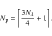
| D | = | (11) | |
| S | = |  |
(12) |
| K | = |  |
(13) |
![\begin{displaymath}\bar{u} = \sqrt[3]{(\ensuremath{\vec{u}_{12}}\!\cdot\!\ensure...
...} )(\ensuremath{\vec{u}_{31}}\!\cdot\!\ensuremath{\vec{i}} )}.
\end{displaymath}](/articles/aa/full/2003/11/aa3304/img52.gif) |
(16) |
![\begin{figure}% latex2html id marker 486\par\includegraphics[width=7.5cm,clip]...
...h{~\ensuremath{{\rm d}^{}\beta}} }_{S D^3}\nonumber
\end{eqnarray} \end{figure}](/articles/aa/full/2003/11/aa3304/img54.gif) |
Figure 2:
Link between the flux distribution
|
| Open with DEXTER | |
The main implication of these results is that the visibility amplitude drop is
a second-order phenomenon (D2u2) while the closure phase is a third-order
one (S D3u3). As a consequence, closure phase is much harder to detect than
the visibility amplitude in a marginally resolved object.
Figure 3 displays the profile of the visibility amplitude and
closure phase as a function of the baseline for a marginally resolved object
with a high asymmetry S = 0.5, as well as the minima of detection for these
quantities as a function of the measurement accuracy. It appears that the
asymmetry is detected for angular sizes 3 to 6 times larger than the spatial
extent or - which is equivalent - for 3 to 6 times larger baselines.
![\begin{figure}
\par\includegraphics[width=5.5cm,clip]{fig3a.eps}\hspace*{4.5mm}
...
....eps}\hspace*{4.5mm}
\includegraphics[width=5.5cm,clip]{fig3c.eps} \end{figure}](/articles/aa/full/2003/11/aa3304/img56.gif) |
Figure 3:
Variation of the square visibility amplitude and closure phase with the
angular size of a marginally resolved object for a 100 m baseline in K,
and the detectability of these quantities. Left panel: square visibility
amplitude vs. angular size; middle panel: closure phase vs. angular size;
right panel: minimum object size needed to detect either the spatial
extent or the asymmetry vs. the instrumental precision on |V|2. On
the first left two view graphs the detection levels for 0.5% and 5%
accuracy on |V|2 measurements are displayed. We assumed
a fairly asymmetric object with S = 0.5, as well as
|
| Open with DEXTER | |
![\begin{figure}
\par\includegraphics[width=6.2cm,clip]{fig4a.eps}\hspace*{2cm}
\includegraphics[width=6.2cm,clip]{fig4b.eps} \end{figure}](/articles/aa/full/2003/11/aa3304/img57.gif) |
Figure 4: Comparison between the exact visibility amplitude of an object and its second-order estimate. Different geometries have been assumed to show that little dependence is found: a symmetrical binary (dashes), a ring (dash-dot-dot), and a Gaussian disc (dots). The left panel displays the second-order estimate (solid line) and the exact visibilities of the different objects vs. the baseline. The right panel displays the visibility amplitude for which an observational difference can be made between the estimate and the exact value vs. the instrumental precision; it is the limit of validity for this estimate. |
| Open with DEXTER | |
![\begin{figure}
\par\includegraphics[width=6.2cm,clip]{fig5a.eps}\hspace*{2cm}
\includegraphics[width=6.2cm,clip]{fig5b.eps} \end{figure}](/articles/aa/full/2003/11/aa3304/img59.gif) |
Figure 5:
Comparison between the exact closure phase of an asymmetrical binary
(
|
| Open with DEXTER | |
The above development presents two limitations: on the one hand, it assumes that all moments are defined and, on the other hand, the first few terms of the series are no longer a good approximation when the object is resolved enough.
In the case of a power law distribution
![]() ,
often
encountered when scattered light dominates, the high-order moments are not
defined. Therefore the above development is no longer valid. For instance,
Lachaume et al. (2003) have shown that a disc with scattering presents a quick drop of
the visibility amplitude near the origin u = 0, that definitely does not present
the smooth profile
,
often
encountered when scattered light dominates, the high-order moments are not
defined. Therefore the above development is no longer valid. For instance,
Lachaume et al. (2003) have shown that a disc with scattering presents a quick drop of
the visibility amplitude near the origin u = 0, that definitely does not present
the smooth profile
![]() .
In Sect. 3.1,
we shall see how to treat scattering at a large scale, while using the above
formalism for other flux contributions.
.
In Sect. 3.1,
we shall see how to treat scattering at a large scale, while using the above
formalism for other flux contributions.
Another important point is the range of validity. The left panel of
Fig. 4 compares the exact visibility of different types of
objects with the second-order estimate (first terms of Eq. (14)) as a
function of the baseline: as expected, the approximation is correct for
under resolved objects with
![]() but gets poorer with larger
baselines. The validity of the approximation depends on whether a difference can
be made between the estimate and the exact value, in other terms whether the
accuracy of the measurement is better than the precision of the estimate. The
right panel of the same figure displays the visibility at which the instrument
accuracy allows us to measure the deviation from the estimate; it appears not to
be much dependent on the geometry of the object. With a typical 2% accuracy
on |V|2, the estimate is valid for
but gets poorer with larger
baselines. The validity of the approximation depends on whether a difference can
be made between the estimate and the exact value, in other terms whether the
accuracy of the measurement is better than the precision of the estimate. The
right panel of the same figure displays the visibility at which the instrument
accuracy allows us to measure the deviation from the estimate; it appears not to
be much dependent on the geometry of the object. With a typical 2% accuracy
on |V|2, the estimate is valid for
![]() .
.
Figure 5 is similar to Fig. 4 but for the
closure phase. For a typical binary with
![]() ,
it displays the
exact closure phase and the third order estimate given in Eq. (15)
as a function of the baseline. The right panel indicates the visibility at
which a differentiation between them can be made as a function of the instrumental
accuracy. With the typical 2% precision on |V|2, the estimate of the phase
is valid for
,
it displays the
exact closure phase and the third order estimate given in Eq. (15)
as a function of the baseline. The right panel indicates the visibility at
which a differentiation between them can be made as a function of the instrumental
accuracy. With the typical 2% precision on |V|2, the estimate of the phase
is valid for
![]() .
.
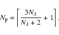
When the accuracy allows us to see the deviation from the third-order estimates, some following orders can be measured and the subsequent moments of the distribution can be accessed. This can be a means to retrieve model-independent spatial information.
![\begin{figure}
\par\includegraphics[width=6.2cm,clip]{fig6a.eps}\hspace*{2cm}
\includegraphics[width=6.2cm,clip]{fig6b.eps} \end{figure}](/articles/aa/full/2003/11/aa3304/img66.gif) |
Figure 6: Point-like source model fitting: number of sources constrained by interferometric observations of a marginally resolved object vs. number of wavelengths used. Left panel: the fluxes at different wavelengths are not correlated. Right panel: the sources are assumed to emit a black-body spectrum. |
| Open with DEXTER | |
Theoretically speaking, the knowledge of visibility and closure phase at all
baselines smaller than B would allow image reconstruction with an infinite
resolution (by using the analycity of the visibility); so, marginal resolution
should not be a problem. This point presents a small but irretrievable flaw:
it assumes that there is no noise in the data. When the finite precision of
measurements is taken into account, the accuracy on the reconstructed image or
model is impaired and also, the number of parameters constrained in a
marginally resolved object. If the visibility amplitude alone is available,
only the quadratic form
![]() can be accessed,
because the deviation from this law cannot be measured, as shown in
Sect. 2.2.
can be accessed,
because the deviation from this law cannot be measured, as shown in
Sect. 2.2.
We first consider an observation carried out at a single wavelength and use the
coordinates (u, v) of ![]() in a Cartesian frame. The visibility amplitude
and phase then are
in a Cartesian frame. The visibility amplitude
and phase then are
| V | = | (17) | |
| = | (18) |
Nevertheless, a multi-wavelength interferometric approach can bring more
constraints. We consider a
![]() point-like source model to be fitted to
visibility amplitudes at
point-like source model to be fitted to
visibility amplitudes at
![]() wavelengths. The fluxes and locations of
the
wavelengths. The fluxes and locations of
the
![]() first sources constrain the last one, because the flux distribution
is normalised and centered; therefore there are
first sources constrain the last one, because the flux distribution
is normalised and centered; therefore there are
![]() locations and
locations and
![]() fluxes, that is
fluxes, that is
![]() free parameters.
Observations provide
free parameters.
Observations provide
![]() moments of the flux distribution. The
characteristic number of point-like sources constrained by the measurements is
given by the equality between the number of free parameters and that of
moments, so that
moments of the flux distribution. The
characteristic number of point-like sources constrained by the measurements is
given by the equality between the number of free parameters and that of
moments, so that
 |
(19) |
 |
(20) |
In conclusion, a multi-wavelength approach allows us to fit more parameters and therefore to distinguish between different scenarios (disc, multiple system, etc.)
![\begin{figure}
\par\includegraphics[width=6.5cm,clip]{fig7.eps} \end{figure}](/articles/aa/full/2003/11/aa3304/img87.gif) |
Figure 7: Visibility curve of an accretion disc. Solid line: all contributions; dashed line: thermal emission of the disc only. |
| Open with DEXTER | |
Circumstellar discs are a good target for interferometers because they scale from a few tens of AU (where they mostly emit thermal light in the infrared) to a few hundreds of AU (where they present scattered light in the infrared) at a typical distance of 150 pc or more. Two issues of interest are: observing their thermal light, because it comes from the first AUs from the star where planets are supposed to form, and deriving their radial temperature law, because it appears as a good diagnosis of the phenomena involved (irradiation, flaring, viscous dissipation, etc.). In Sect. 3.1 we show how to take into account both the thermal and scattered light, which happen to present different interferometric signatures. In Sect. 3.2, we establish a connection between the temperature law and the wavelength dependence of the visibility.
Describing an accretion disc as a marginally resolved object is inaccurate
because thermal light occurs at a large scale and accounts for up to 10% of
the total flux. In order to keep the above formalism, we split the image into
three components: stellar contribution, thermal emission of the disc, and
scattered light. To each contribution, one can associate a corresponding
visibility:
| |
= | (21) | |
| = |  |
(22) | |
| = |  |
(23) |
We assumed that both the star and the thermal emission of the disc are marginally
resolved, that the scattering emission is fully resolved as soon as the
baseline is non-zero, and that the star is too small and symmetric to present a
phase. Within the approximation that all components have the same photocentre,
we derive the total visibility
 |
(24) |
From visibilities at different wavelengths, Malbet & Berger (2002a) showed that
the temperature profile of an accretion disc can be derived. In the
context of a massive disc, the flux is dominated by thermal light so
that
 |
(25) |
 |
(27) |
| |
= | (28a) | |
| = | 0, | (28b) | |
| (28c) |
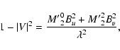
| (29) | |||
| 1-|V|2 | (30) |
![\begin{figure}
\par\includegraphics[width=6.2cm,clip]{fig8a.eps}\hspace*{2cm}
\includegraphics[width=6.2cm,clip]{fig8b.eps} \end{figure}](/articles/aa/full/2003/11/aa3304/img120.gif) |
Figure 8:
Apparent temperature law, given by the exponent
|
| Open with DEXTER | |
Note that the result no longer holds when the disc presents an inner
hole. Figure 8 displays the value
![]() deduced from
Eq. (31) with the H and K bands for a typical FU Ori disc. The
parameters of the disc model are given in Appendix D.
When the inner gap becomes larger than a few stellar radii, the error on q,
deduced from
Eq. (31) with the H and K bands for a typical FU Ori disc. The
parameters of the disc model are given in Appendix D.
When the inner gap becomes larger than a few stellar radii, the error on q,
![]() can be larger than 0.1. Malbet & Berger (2002a) find
can be larger than 0.1. Malbet & Berger (2002a) find
![]() for FU Ori; with a typical value
for FU Ori; with a typical value
![]() (Lachaume et al. 2003),
we can estimate
(Lachaume et al. 2003),
we can estimate
![]() from the curves.
from the curves.
The stellar radius has also an influence because of the unresolved stellar flux, yet, it remains small for FU Ori discs (see Fig. 8). In the case of a T Tauri star, the error could be much larger, because the contribution of the star to the total flux becomes important.
We have developed a formalism that connects the visibility amplitude and phase of a marginally resolved object with its geometry, namely the moments of the flux distribution. It can prove particularly useful when constraining models that present analytical moments and allows us to retrieve model-independent spatial information in all cases. It also establishes that the closure phase of a marginally resolved source is a third-order term and the visibility a second-order one; therefore, the phase is much harder to detect than the drop in visibility amplitude.
From the formalism, we were also able to estimate the number of parameters relevantly fitted to interferometric measurements. Unless observations are carried out at several wavelengths and the model assumes a black-body-like emission, only a few parameters can be fitted to marginally resolved objects, whatever the number of visibility points taken: three point-like source with visibility amplitudes only, and a fourth one if closure phase is also measured. This limitation is removed when the object is more resolved, that is, if the baselines are longer or if the instrumental accuracy is increased, which allows us to measure the deviation of the visibility and phase from their low-order estimates. This work can therefore be seen as a plea for larger baselines than the CHARA array provides, or high accuracy with IOTA/IONIC or the forthcoming VLTI and Keck.
We then applied this theoretical work to circumstellar discs, by separating the star, the thermal emission of the disc, and the scattered light, the two first ones being well described by their moments. It also allows us to derive, with some hypotheses, information on the radial temperature law in these objects, even if they are underresolved, but requires that measurements should be taken at two or more wavelengths. This can be applied to other field. For instance, limb-darkened stellar photospheres can be probed even with underresolved targets: the equivalent diameter is dependent on the wavelength and one could, with an appropriate model, measure this darkening.
With high precision measurements and/or multiple wavelengths one can access a large number of moments of the flux distribution, which theoretically allows image reconstruction. This is clearly a path that one should investigate in the near future. As a particular case, we believe it is possible to retrieve the radial temperature profile of supposedly symmetrical objects, as as been initiated with FU Ori. The method could also prove useful to constrain the location of stellar spots with high accuracy measurements: the link between the location of these spots and the first order moments of the flux is much clearer than the information given by image reconstruction techniques.
Acknowledgements
I thank Fabien Malbet, Jean-Philippe Berger, and Jean-Baptiste Lebouquin for helpful discussions; without their interest, this work would have stayed hidden under a heavy stack on my desk. Computations and graphics have mostly been carried out with the free software Yorick by D. Munro. Useful comments from Theo ten Brummelaar led to an improved presentation of these results.
We use a Cartesian frame in which
![]() has coordinates
has coordinates
![]() throughout this appendix.
throughout this appendix.
The first moment is a vector
 |
(A.1) |
| M10 | = | (A.2a) | |
| M11 | = | (A.2b) |
![\begin{displaymath}\vec{M}_2 = \left(
\begin{array}{ll}
M_2^0 & M_2^1\\ [2mm]
M_2^1 & M_2^2
\end{array} \right)
\end{displaymath}](/articles/aa/full/2003/11/aa3304/img129.gif) |
(A.3) |
| M20 | = | (A.4a) | |
| M21 | = | (A.4b) | |
| M22 | = | (A.4c) |
 |
(A.5) |
We define
| J1 | = | (B.1) | |
| Jn | = |  |
(B.2) |
| V | = |  |
|
 |
|||
 |
(B.3) | ||
| (B.4) | |||
| = |  |
||
 |
|||
 |
|||
| (B.5) |
We consider a face-on disc with a radial temperature law
![]() ,
where r is the angular distance from the centre. The flux distribution
then reads
,
where r is the angular distance from the centre. The flux distribution
then reads
 |
(C.1) |
 |
(C.5) |
| |
= | I3/(2I1), | (C.7) |
| = | 0, | (C.8) | |
| = | I3/(2I1). | (C.9) |
 |
(C.10) |
 |
(C.11) |
 |
(C.12) |
 |
(C.13) |
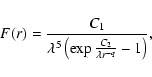
The FU Ori disc model has been determined with an effective temperature
T(r)
= K r-q. The influence of the central gap or of the star highly
depends on the constant K. In the standard viscous disc model (q = 3/4) by
Shakura & Sunyaev (1973),
![\begin{displaymath}K = \sqrt[4]{\frac{3\mathcal{G}\ensuremath{M_*}\ensuremath{\dot M} }{8\sigma\pi}},
\end{displaymath}](/articles/aa/full/2003/11/aa3304/img163.gif) |
(D.1) |
 |
(D.2) |
| |
= | (D.3a) | |
| = | (D.3b) |
![\begin{displaymath}q = \frac{1}{\displaystyle 1+ \frac12 \frac{\log [(1-\vert V_...
...t^2)/(1-\vert V_2\vert^2)]}
{\log [\lambda_2/\lambda_1]}}\cdot
\end{displaymath}](/articles/aa/full/2003/11/aa3304/img117.gif)