A&A 398, 159-168 (2003)
DOI: 10.1051/0004-6361:20021626
A. J. Gawryszczak -
J. Miko![]() ajewska -
M. Rózyczka
ajewska -
M. Rózyczka
Nicolaus Copernicus Astronomical Center, Bartycka 18, Warsaw 00-716, Poland
Received 28 August 2002 / Accepted 25 October 2002
Abstract
The slow and dense wind from a symbiotic red giant (RG)
can be significantly deflected toward the orbital plane by the gravitational
pull of the companion star. In such an environment, the ionizing radiation
from the companion creates a highly asymmetric H II region. We present
three-dimensional models of H II regions in symbiotic S-type systems,
for which we calculate radio maps and radio spectra. We show that the
standard assumption of spherically symmetric RG wind results in wrong shapes,
sizes and spectra of ionized regions, which in turn affects the observational
estimates of orbital separation and mass loss rate. A sample of radio maps
and radio spectra of our models is presented and the results are discussed in
relation to observational data.
Key words: stars: winds, outflows - stars: binaries: symbiotic - hydrodynamics
Radio emission from symbiotic stars is dominated by ff radiation
from the ionized gas. The ff spectrum of an H II region
consists of three parts: optically thick at low frequencies (with
spectral index
![]() ), optically thin at high frequencies
(with
), optically thin at high frequencies
(with
![]() ), and optically semi-thick at intermediate
frequencies around a turnover frequency
), and optically semi-thick at intermediate
frequencies around a turnover frequency
![]() ,
with
,
with
![]() smoothly decreasing from its optically thick value to
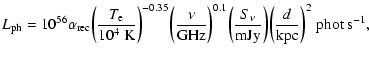
-0.1. Taylor & Seaquist (1984) show that orbital separation a, ionizing
luminosity
smoothly decreasing from its optically thick value to
-0.1. Taylor & Seaquist (1984) show that orbital separation a, ionizing
luminosity
![]() ,
and the ratio of mass-loss rate to wind
velocity
,
and the ratio of mass-loss rate to wind
velocity
![]() may be derived from such observables as
turnover frequency, monochromatic flux at that frequency
may be derived from such observables as
turnover frequency, monochromatic flux at that frequency
![]() ,
and the value of the optically thick spectral index.
,
and the value of the optically thick spectral index.
However, their calculations are based on the spherical wind model originally developed by Seaquist et al. (1984) (hereafter STB), which, as we mentioned above, is incorrect in closer systems. Good examples of such systems are symbiotic S-type systems, containing a normal M giant and having orbital periods of order a few years (e.g. Belczynski et al. 2000, and references therein).
Recently, Miko![]() ajewska & Ivison (2001) have obtained for the first time the spectral
energy distribution (SED) at wavelengths between
ajewska & Ivison (2001) have obtained for the first time the spectral
energy distribution (SED) at wavelengths between
![]() and
and
![]() for one of the prototypical S-type systems,
CI Cyg, during quiescence. Their data allowed to determine
for one of the prototypical S-type systems,
CI Cyg, during quiescence. Their data allowed to determine
![]() and the optically thin ff emission measure, from which
a lower limit to
and the optically thin ff emission measure, from which
a lower limit to
![]() and an estimate of a were
calculated within the STB framework. Unfortunately, the comparison of
these estimates with the known orbital and stellar parameters of
CI Cyg poses a serious problem for the STB model. In
particular, a is overestimated by a factor of
and an estimate of a were
calculated within the STB framework. Unfortunately, the comparison of
these estimates with the known orbital and stellar parameters of
CI Cyg poses a serious problem for the STB model. In
particular, a is overestimated by a factor of ![]() 35, whereas
35, whereas
![]() (whose value is known from optical/UV H I
emission lines and He II bf+ff continuum) is
underestimated by a factor of
(whose value is known from optical/UV H I
emission lines and He II bf+ff continuum) is
underestimated by a factor of ![]() 20.
20.
The above inconsistency strongly indicates that the STB model needs
revision. The most obvious improvements are related to the asphericity
of the wind, as suggested both by numerical work
(see Gawryszczak et al. 2002, and references therein) and observations. From the
observational point of view there is little doubt about the origin of
the ionized medium. The mm radio emission shows some correlation with
the mid-IR flux, and the radio luminosity increases with the
![]() colour. This indicates that warm dust is involved in
the mass flow along with the ionized gas, and suggests that the red
giant is the source of this material (Miko
colour. This indicates that warm dust is involved in
the mass flow along with the ionized gas, and suggests that the red
giant is the source of this material (Miko![]() ajewska et al. 2002a). Such a picture is
also supported by the spectral analysis of symbiotic nebulae which
showed CNO abundances similar to those observed in normal red giants
(Nussbaumer et al. 1988) Optical and radio imaging of symbiotic stars reveal
aspherical nebulae, often with bipolar lobes and jet-like components
(Corradi et al. 1999). It is hard to explain how such structures might
develop if the RG wind were spherical. Additional, indirect evidence
for the asphericity of the RG wind comes from emission line
profiles. It is based on the stationary, blueshifted
ajewska et al. 2002a). Such a picture is
also supported by the spectral analysis of symbiotic nebulae which
showed CNO abundances similar to those observed in normal red giants
(Nussbaumer et al. 1988) Optical and radio imaging of symbiotic stars reveal
aspherical nebulae, often with bipolar lobes and jet-like components
(Corradi et al. 1999). It is hard to explain how such structures might
develop if the RG wind were spherical. Additional, indirect evidence
for the asphericity of the RG wind comes from emission line
profiles. It is based on the stationary, blueshifted
![]() absorption originating close to the orbital plane
and indicating that the ionized region is probably bounded on all
sides by a significant amount of dense neutral material (see the
discussion in Gawryszczak et al. 2002).
absorption originating close to the orbital plane
and indicating that the ionized region is probably bounded on all
sides by a significant amount of dense neutral material (see the
discussion in Gawryszczak et al. 2002).
In the present paper we account for the asphericity of the RG as resulting from the interaction with the secondary. With the help of 3-D hydrodynamical models we demonstrate that H II regions ionized by the secondary in S-type systems must indeed have shapes, sizes and spectra significantly different from those obtained by STB. A representative sample of radio spectra and radio maps of our models is also generated.
In Sect. 2 we discuss the numerical techniques used in this work and details of the physical setup of our models. The models are presented in Sect. 3. In Sect. 4 the results of our simulations are compared to observed symbiotic systems and a brief summary of our work is provided.
We begin with 3-D hydrodynamical simulations of RG winds interacting with the companion to the mass-losing star. The simulations are performed with the help of the Smoothed Particle Hydrodynamics (SPH) technique. An inertial coordinate system is used, with the origin at the mass center of the binary.
Our implementation of the SPH is based on variable smoothing length
with spline kernel introduced by Monaghan & Lattanzio (1985). The number of
neighbouring particles is set to 40. For practical reasons (CPU
time), the total number of particles in the computational domain is
limited to 105. Whenever this limit is exceeded, those most distant
from the system are removed from the domain. The distance beyond which
removals occur (
![]() )
stabilizes within several orbital
periods of the binary, and an almost stationary rotating density
distribution is obtained. The validity of such an approach was
demonstrated by Gawryszczak et al. (2002). With the above limit imposed on the
number of particles,
)
stabilizes within several orbital
periods of the binary, and an almost stationary rotating density
distribution is obtained. The validity of such an approach was
demonstrated by Gawryszczak et al. (2002). With the above limit imposed on the
number of particles,
![]() does not exceed
does not exceed
![]() (see Table 1).
(see Table 1).
Within
![]() from the secondary
we remove all particles with velocities directed toward the secondary.
This procedure is applied to avoid prohibitively short time-steps.
from the secondary
we remove all particles with velocities directed toward the secondary.
This procedure is applied to avoid prohibitively short time-steps.
There are good reasons to believe that RG winds are intrinsically aspherical
(see e.g. Frankowski & Tylenda 2001; Dorfi & Höfner 1996; Reimers et al. 2000, and references therein). The
asphericity may result from internal processes taking place in the
star and/or presence of the secondary. However, since the theory is
not yet advanced enough for precise quantitative predictions, these
effects are not included in our models. In particular, we assume that
although the RG rotates synchronously it does not fill its Roche lobe,
so that the mass flow through the inner Lagrangian point can be
neglected. In effect, the wind is represented by a stream of particles
launched at a constant rate from points distributed randomly and
uniformly on the RG surface. The initial temperature of the wind is
![]() ,
and the initial velocity of wind particles is set
to
,
and the initial velocity of wind particles is set
to
![]() (note that, as the wind propagates across
the grid its velocity increases; a measure of the terminal wind velocity
is introduced and explained in the following paragraphs).
Both temperature and velocity of the wind
are constant on the surface of the star.
(note that, as the wind propagates across
the grid its velocity increases; a measure of the terminal wind velocity
is introduced and explained in the following paragraphs).
Both temperature and velocity of the wind
are constant on the surface of the star.
Further, we assume that the wind is composed of dust and ideal monoatomic gas which are dynamically coupled (i.e. they move at the same velocity). The details of wind acceleration process are not followed. Instead, we assume that the gravity of the red giant is balanced by radiation pressure on the dust, so that it does not appear explicitly in our equations. Thus, if the RG were single, the only force acting on the wind would be due to gas-pressure gradients, whereas in a binary the wind is additionally subject to the gravity of the companion. Such an approximation may seem rather crude; however Gawryszczak et al. (2002) demonstrated that it leads to terminal velocities comparable to those obtained by Winters et al. (2000) for winds in which radiation pressure nearly balances the gravity of the wind source.
Finally, we neglect radiation pressure from the secondary
(note that in the case of a white dwarf,for any reasonable grain size the
force due to radiation pressure on dust grains is much smaller than gravity).
Self-gravity of the wind and any explicit radiative heating or
cooling are also neglected. The effects of cooling are accounted for by a
nearly isothermal equation of state employed for the wind (
![]() ,
with
,
with
![]() ).
A likely source of strong nonaxisymmetric effects is magnetic field, as the
MHD collimation may be much more efficient than the gravitational focusing
discussed here (see García-Segura et al. 1999; García-Segura & López 2000; García-Segura et al. 2001, and references therein).
However, there is
no information available about magnetic fields in symbiotic systems and we
feel that it is too early to incorporate them into models: the number of free
parameters would simply grow too large.
).
A likely source of strong nonaxisymmetric effects is magnetic field, as the
MHD collimation may be much more efficient than the gravitational focusing
discussed here (see García-Segura et al. 1999; García-Segura & López 2000; García-Segura et al. 2001, and references therein).
However, there is
no information available about magnetic fields in symbiotic systems and we
feel that it is too early to incorporate them into models: the number of free
parameters would simply grow too large.
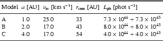
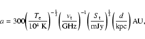
All binaries considered here consist of a
![]() red giant and a
red giant and a
![]() white dwarf. The orbital separation a varies between 1 and
white dwarf. The orbital separation a varies between 1 and
![]() ,
which is representative of S-type symbiotic systems.
Following Miko
,
which is representative of S-type symbiotic systems.
Following Miko![]() ajewska et al. (2002a) a mass loss rate of
ajewska et al. (2002a) a mass loss rate of
![]() is adopted for the RG wind,
while the ionizing luminosity of the secondary
is adopted for the RG wind,
while the ionizing luminosity of the secondary
![]() varies
between
varies
between
![]() and
and
![]() .
The
latter range is compatible with estimates based on mm/submm observations
(Ivison & Seaquist 1995; Miko
.
The
latter range is compatible with estimates based on mm/submm observations
(Ivison & Seaquist 1995; Miko![]() ajewska & Ivison 2001), but is a factor of
ajewska & Ivison 2001), but is a factor of ![]() 10 smaller than estimates based
on studies of optical/UV H I and He II emission lines and
bf+ff continuum (Miko
10 smaller than estimates based
on studies of optical/UV H I and He II emission lines and
bf+ff continuum (Miko![]() ajewska & Ivison 2001; Miko
ajewska & Ivison 2001; Miko![]() ajewska et al. 2002a).
ajewska et al. 2002a).
The choice of the lower estimate is dictated by the size of our
hydrodynamical wind models (
![]() in diameter),
which at
in diameter),
which at
![]() would be practically entirely
ionized. The parameters of symbiotic binary models obtained in this
work are listed in Table 1 (
would be practically entirely
ionized. The parameters of symbiotic binary models obtained in this
work are listed in Table 1 (
![]() in Col. 3
is a measure of the wind velocity; see Sect. 3.2 for
an explanation). The radius of the red giant is in all cases equal to
in Col. 3
is a measure of the wind velocity; see Sect. 3.2 for
an explanation). The radius of the red giant is in all cases equal to
![]() .
A simple method of scaling our results to
combinations of
.
A simple method of scaling our results to
combinations of ![]() and
and
![]() not covered by actual
calculations is given in Sect. 3.3.
not covered by actual
calculations is given in Sect. 3.3.
![\begin{figure}
\par\includegraphics[width=13cm,clip]{aa3046f1.eps}\par\end{figure}](/articles/aa/full/2003/04/aa3046/img53.gif) |
Figure 1:
Density distributions of models A, B and C. The logarithmic density
scale spans 5 orders of magnitude. In each frame a region of
|
| Open with DEXTER | |
All models also display a three-dimensional spiral structure resulting from the shock wave excited by the motion of the secondary across the RG wind. The spirals are a very general feature of slow winds in binary systems, and they were also observed in simulations reported by Mastrodemos & Morris (1998, 1999) or Gawryszczak et al. (2002). As one might expect, in closer binaries the spiral is more tightly wound than in the wider ones.
In the closest binary funnel-like density minima oriented perpendicularly to the orbit are also observed. Two effects contribute to the formation of these funnels. First, in a close binary the wind is emitted from a source moving with a high orbital velocity, and as such it carries appreciable angular momentum. Away from the orbital plane the centrifugal force associated with that momentum causes the wind gas to clear the vicinity of the polar axis. Secondly, and unlike that of the primary, the gravity of the secondary is not balanced by radiation pressure, and the wind flowing perpendicularly to the orbit is retarded.
Below we argue that all these features (flattening, spirals and funnels) are important factors influencing the observational properties of the H II regions created in the RG wind by the ionizing radiation from the secondary.
Once the RG wind has been relaxed, its density distribution is smoothed by averaging over several tens of consecutive time steps. The aim of this procedure is to reduce the numerical noise resulting from the "grainy" nature of the SPH models. The smoothed density is mapped onto a spherical grid centered on the secondary, with grid points spaced uniformly in angular coordinates and concentrated at the secondary in the radial coordinate. Then, the source of ionizing photons is turned on at the location of the secondary, and the boundary of the H II region is found in a local Strömgren sphere approximation (i.e. Strömgren radii are calculated for all directions defined by grid points in angular coordinates). An example result of this procedure is shown in Fig. 2. Separate treatment of ionization and dynamics is justified by the fact that the recombination time is one order of magnitude shorter than the orbital period at the edge of our computational domain, and more than 3 orders of magnitude near the secondary.
In the approach developed by STB, the shape and size of the H II
region are uniquely determined by the value of the parameter X,
which is a combination of the mass loss rate, wind velocity, orbital
separation, and ionizing luminosity:
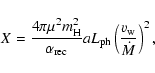 |
(1) |
While STB assume a wind of constant velocity, in our models the flow
accelerates with the distance from the RG, and the acceleration
proceeds at a variable (location-dependent) rate. This is due partly
to thermal pressure gradients, and partly to the centrifugal force
associated with the angular momentum transferred to the wind from the
secondary; see
Gawryszczak et al. (2002). In order to calculate X from our models, we use a
density-weighted velocity
![]() ,
averaged over the whole
solid angle (the averaging is performed near the edge of the
computational domain). For each binary a range of H II regions
with different X-values may then be easily generated by allowing
for variations in
,
averaged over the whole
solid angle (the averaging is performed near the edge of the
computational domain). For each binary a range of H II regions
with different X-values may then be easily generated by allowing
for variations in
![]() (alternatively,
(alternatively, ![]() may be
scaled by multiplying the density of the RG wind in each grid cell by
the same factor).
may be
scaled by multiplying the density of the RG wind in each grid cell by
the same factor).
To obtain the STB counterpart of our model, for the same ![]() a
density distribution of the spherical wind from the primary is
calculated, assuming
a
density distribution of the spherical wind from the primary is
calculated, assuming
![]() .
An appropriate part
of that distribution is fed into the spherical grid centered on the
secondary, and the same Strömgren-routine is employed to find the
boundary of H II region. We checked that the boundary found
this way agrees to within a few percent with the boundary derived from
Eq. (1) of STB.
.
An appropriate part
of that distribution is fed into the spherical grid centered on the
secondary, and the same Strömgren-routine is employed to find the
boundary of H II region. We checked that the boundary found
this way agrees to within a few percent with the boundary derived from
Eq. (1) of STB.
 |
Figure 2:
3D view of the H II region boundary in model B with
|
| Open with DEXTER | |
The two sets of H II regions are compared in Fig. 3. The upper part of each frame shows our model, and the lower one - the corresponding model obtained within the framework of STB (note that all displayed models are symmetric with respect to the orbital plane).
A clear general trend may be observed: for wide binaries and intense ionizing
fluxes (see lower right corner of Fig. 3) the shapes and
sizes of our H II regions converge to those of STB. On the other hand,
for close binaries and/or low ionizing luminosities, our H II regions
become entirely different from those of STB: they are not axially symmetric,
and their shapes may be fairly complicated (see Fig. 2 and the
left column of Fig. 3). Another discrepancy concerns a
large part of the space to the right of the secondary in
Fig. 3, which in our models is screened from UV photons by
the dense disk around the secondary. This neutral region, best visible in the
upper right frames of Fig. 3, does not have its
counterpart in STB models, and it only disappears when
![]() is
large enough to ionize the disk.
is
large enough to ionize the disk.
Note also that our H II regions are generally smaller than those of
STB. This is due to the fact that the density of our RG wind is enhanced in
the orbital plane compared to the spherically symmetric wind with the same
mass loss rate and velocity. However, in the closest binary with the lowest
![]() our H II region becomes much larger than its STB
counterpart. This is because the low-density funnels, which are very well
developed in this case, are easily ionized, causing the H II region to
evolve into a pair of semi-infinite jet-like lobes (upper left frame of
Fig. 3).
our H II region becomes much larger than its STB
counterpart. This is because the low-density funnels, which are very well
developed in this case, are easily ionized, causing the H II region to
evolve into a pair of semi-infinite jet-like lobes (upper left frame of
Fig. 3).
![\begin{figure}
\includegraphics[width=13cm,clip]{aa3046f3.eps} \end{figure}](/articles/aa/full/2003/04/aa3046/img64.gif) |
Figure 3:
A sample of H II region shapes. H II region boundary
is plotted in a plane which is perpendicular to the orbit and contains
the centers of both stars. In every frame our model (top) is compared to
its STB counterpart (bottom) obtained for the same value of X. The
columns illustrate the effect of increasing luminosity, (or,
equivalently, of increasing X). In each frame a region of
|
| Open with DEXTER | |
The resulting spectra of all models presented in Fig. 3
are displayed in Fig. 4 (note that in both figures the
models are arranged in the same way, but the whole Fig. 4
is rotated counterclockwise by 90
![]() ). For comparison, the corresponding
STB spectra are also shown. All spectra may easily be scaled to other values
of
). For comparison, the corresponding
STB spectra are also shown. All spectra may easily be scaled to other values
of ![]() and
and
![]() ;
the corresponding procedure is illustrated
in Fig. 5.
;
the corresponding procedure is illustrated
in Fig. 5.
As one might expect, in wider systems with high
![]() our spectra
almost entirely converge to those of STB, while they are significantly
different in close systems with low
our spectra
almost entirely converge to those of STB, while they are significantly
different in close systems with low
![]() .
In such systems our
spectral index may be smaller or larger than that of STB; the same is true
for turnover frequency and intensity. To make things even more complicated,
some spectra exhibit more than one turnover. This is because in some models
the distribution of density along the line of sight cannot be approximated by
a single power law.
.
In such systems our
spectral index may be smaller or larger than that of STB; the same is true
for turnover frequency and intensity. To make things even more complicated,
some spectra exhibit more than one turnover. This is because in some models
the distribution of density along the line of sight cannot be approximated by
a single power law.
In general, the differences between the spectra of the same system viewed "pole-on'' and along the line joining the stars (with the primary in front of the secondary) are larger in our models than in those of STB (slopes and turnover frequencies are however almost insensitive to such a change of viewing direction). On the other hand, our models predict weaker spectral variations with the orbital phase. This behaviour is explained by the fact that in our models the distinguished direction is perpendicular to the orbital plane, whereas the H II regions of STB are axially symmetric with respect to the line joining the stars.
![\begin{figure}
\par\mbox{
\includegraphics[angle=90,width=3.4cm,clip]{aa3046f4L...
...m}
\includegraphics[angle=90,width=4.15cm,clip]{aa3046f4Rc.eps} }
\end{figure}](/articles/aa/full/2003/04/aa3046/img72.gif) |
Figure 4:
Radio spectra of models shown in Fig. 3. In all
cases
|
| Open with DEXTER | |
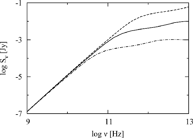 |
Figure 5:
Scaling of the spectra. Compared are variants of model B with
|
| Open with DEXTER | |
The bipolar structure shown by our maps could be easily resolved by MERLIN
after its upgrade is complete (e-MERLIN). Even now, MERLIN has sufficient
resolution (
![]() at
at
![]() where it is most
sensitive) but its sensitivity is too low. However, e-MERLIN, with its new 15
and
where it is most
sensitive) but its sensitivity is too low. However, e-MERLIN, with its new 15
and
![]() receivers will be able to perform imaging at a
resolution of
receivers will be able to perform imaging at a
resolution of ![]() 8 AU at
8 AU at
![]() for sources as weak
as a few of
for sources as weak
as a few of
![]() .
.
![\begin{figure}
\par {
\includegraphics[width=4cm,clip]{3046f6a1.eps}\hspace*{1....
...}\hspace*{1.4cm}
\includegraphics[width=4cm,clip]{3046f6c5.eps} }
\end{figure}](/articles/aa/full/2003/04/aa3046/img92.gif) |
Figure 6:
Selected radiomaps at
|
| Open with DEXTER | |
In systems with ![]() and
and ![]() our radio spectra significantly
diverge from those of STB. First, the location and extent of the
transition region between optically thin and optically thick parts of
the spectrum are different. Second, the shape of the transition region
is more complicated in our models. Third, our models radiate much less
energy in the optically thick part of the spectrum than their STB
counterparts (the difference can amount to two orders of magnitude).
our radio spectra significantly
diverge from those of STB. First, the location and extent of the
transition region between optically thin and optically thick parts of
the spectrum are different. Second, the shape of the transition region
is more complicated in our models. Third, our models radiate much less
energy in the optically thick part of the spectrum than their STB
counterparts (the difference can amount to two orders of magnitude).
The latter result can be understood as a simple consequence of the
smaller spatial extent of our H II regions (the optically thick
flux is roughly proportional to the projected surface area of the
ionized part of the wind). In principle, the remaining predictions
could be verified by spectroscopic observations. Unfortunately,
observational data, especially at higher frequencies, are still too
poor to discriminate between various theoretical models. The broadest
survey available, reported by Miko![]() ajewska et al. (2002a,b) is based on
mm/submm observations of a sample of 20 S-type systems in
quiescence. Radio emission from these systems is found to be optically
thick at least up to
ajewska et al. (2002a,b) is based on
mm/submm observations of a sample of 20 S-type systems in
quiescence. Radio emission from these systems is found to be optically
thick at least up to ![]() 1.3 mm
1.3 mm
![]() = turnover frequency). This is compatible both with the STB
model, which for typical quiescent S-type systems predicts
= turnover frequency). This is compatible both with the STB
model, which for typical quiescent S-type systems predicts
![]() (Seaquist et al. 1993), and with our
simulations (see Fig. 4).
(Seaquist et al. 1993), and with our
simulations (see Fig. 4).
At present the only system which allows for a quantitative analysis of
the spectrum is
CI Cyg, where
![]() .
For
the STB model the outcome of such an analysis is rather
unfavourable. In their framework the orbital separation may be
estimated from
.
For
the STB model the outcome of such an analysis is rather
unfavourable. In their framework the orbital separation may be
estimated from
The STB framework also provides an estimate for
![]()
Other inconsistencies between the observed spectrum of CI Cyg and
the STB model are discussed by Miko![]() ajewska & Ivison (2001), who suggest that the STB approach
might not apply to this system because it is likely that the red giant fills
or nearly fills its Roche lobe, and the mass loss is concentrated in a stream
flowing through the inner Lagrangian point. If this is really the case, then
our models, which predict concentration of the outflow in the equatorial
plane and formation of the circumsecondary disk, should provide a better
approximation of the observed spectrum than that obtained within the STB
framework.
ajewska & Ivison (2001), who suggest that the STB approach
might not apply to this system because it is likely that the red giant fills
or nearly fills its Roche lobe, and the mass loss is concentrated in a stream
flowing through the inner Lagrangian point. If this is really the case, then
our models, which predict concentration of the outflow in the equatorial
plane and formation of the circumsecondary disk, should provide a better
approximation of the observed spectrum than that obtained within the STB
framework.
Unfortunately, in this particular system they do not perform much better.
A glance at Fig. 4 indicates that in order to obtain
![]() as low as
as low as ![]() 30 GHz we would have to assume
an unacceptably low
30 GHz we would have to assume
an unacceptably low
![]() and/or
and/or ![]() much lower than
much lower than
![]() .
A likely solution to this problem is suggested by the spectrum for
.
A likely solution to this problem is suggested by the spectrum for
![]() in Fig. 4, which is the only
one showing an excess in the optically thick part. With increasing
in Fig. 4, which is the only
one showing an excess in the optically thick part. With increasing ![]() and
and
![]() the excess would shift to higher frequencies, mimicking
the turnover observed in CI Cyg. The fact that the spectrum obtained
for
the excess would shift to higher frequencies, mimicking
the turnover observed in CI Cyg. The fact that the spectrum obtained
for
![]() offers a better fitting possibility for the system
with
offers a better fitting possibility for the system
with
![]() seems to indicate that our model of the latter
underestimates the density of the circumsecondary disk and/or overestimates
the density of the funnels. Such a conclusion is compatible with arguments
concerning the outflow through the inner Lagrangian point.
The deciding tests of our results will become possible when high-resolution
radio maps of S-type systems are obtained. Our results suggest that S-type
systems will be interesting targets for e-MERLIN and ALMA.
seems to indicate that our model of the latter
underestimates the density of the circumsecondary disk and/or overestimates
the density of the funnels. Such a conclusion is compatible with arguments
concerning the outflow through the inner Lagrangian point.
The deciding tests of our results will become possible when high-resolution
radio maps of S-type systems are obtained. Our results suggest that S-type
systems will be interesting targets for e-MERLIN and ALMA.
While the models presented here are closer to reality than those obtained
within the STB approach, there is still a considerable room for improvements.
We have only marginally resolved the disk around the secondary, whose shape
and extent may strongly influence shape and extent of the H II region.
To improve on that, future work should include effects of radiation transfer
and viscosity, increase the mass-resolution of the SPH code and,
accordingly, decrease its time-step. Note, however, that with radiation
transfer and viscosity included, the simple scaling relation presented in
Fig. 5 would not work. This means that RG wind
models extending to hundreds of ![]() would have to be obtained in
order to generate H II regions emitting as much energy in the
optically thin regime as the observed ones. Such simulations would push the
CPU requirements beyond currently acceptable limits. When they are hopefully
done in the future and a reliable thermal structure of the flow is obtained,
the thermal ionization should be taken into account, which at least in some
cases may significantly contribute to the radio spectra.
would have to be obtained in
order to generate H II regions emitting as much energy in the
optically thin regime as the observed ones. Such simulations would push the
CPU requirements beyond currently acceptable limits. When they are hopefully
done in the future and a reliable thermal structure of the flow is obtained,
the thermal ionization should be taken into account, which at least in some
cases may significantly contribute to the radio spectra.
Acknowledgements
This research was supported by the Committee for Scientific Research through grants 2P03D 014 19 and 5P03D 019 20.