A&A 398, 49-61 (2003)
DOI: 10.1051/0004-6361:20021620

The FORS Deep Field: Field selection, photometric observations and photometric catalog^,

J. Heidt¹ - I. Appenzeller¹ - A. Gabasch² - K. Jäger³ - S. Seitz² - R. Bender² - A. Böhm³ - J. Snigula² - K. J. Fricke³ - U. Hopp² - M. Kümmel⁴ - C. Möllenhoff¹ - T. Szeifert⁵ - B. Ziegler^3,6 - N. Drory² - D. Mehlert¹ - A. Moorwood⁷ - H. Nicklas³ - S. Noll¹ - R. P. Saglia² - W. Seifert¹ - O. Stahl¹ - E. Sutorius^1,8 - S. J. Wagner¹

1 - Landessternwarte Heidelberg, Königstuhl, 69117 Heidelberg, Germany
2 - Universitätssternwarte München, Scheinerstr. 1, 81679 München, Germany
3 - Universitäts-Sternwarte Göttingen, Geismarlandstr. 11, 37083 Göttingen, Germany
4 - Max-Planck-Institut für Astronomie, Königstuhl 17, 69117 Heidelberg, Germany
5 - European Southern Observatory Santiago, Alonso de Cordova 3107, Santiago 19, Chile
6 - Akademie der Wissenschaften, Theaterstr. 7, 37079 Göttingen, Germany
7 - European Southern Observatory, Karl-Schwarzschild-Str. 2, 85748 Garching, Germany
8 - Royal Observatory Edinburgh, Blackford Hill, Edinburgh EH9 3HJ, UK

Received 11 July 2002 / Accepted 15 October 2002

Abstract
The FORS Deep Field project is a multi-colour, multi-object spectroscopic investigation of a $\sim$ $7\hbox{$^\prime$ }\times 7\hbox{$^\prime$ }$ region near the south galactic pole based mostly on observations carried out with the FORS instruments attached to the VLT telescopes. It includes the QSO Q 0103-260 (z = 3.36). The goal of this study is to improve our understanding of the formation and evolution of galaxies in the young Universe. In this paper the field selection, the photometric observations, and the data reduction are described. The source detection and photometry of objects in the FORS Deep Field is discussed in detail. A combined B and I selected UBgRIJKs photometric catalog of 8753 objects in the FDF is presented and its properties are briefly discussed. The formal 50% completeness limits for point sources, derived from the co-added images, are 25.64, 27.69, 26.86, 26.68, 26.37, 23.60 and 21.57 in U, B, g, R, I, J and Ks (Vega-system), respectively. A comparison of the number counts in the FORS Deep Field to those derived in other deep field surveys shows very good agreement.

Key words: methods: data analysis - catalogs - galaxies: general - galaxies: fundamental parameters - galaxies: photometry

1 Introduction

Deep field studies have become one of the most powerful tools to explore galaxy evolution over a wide redshift range. One of the main aims of this kind of study is to constrain current evolutionary scenarios for galaxies, such as the hierarchical structure formation typical of Cold Dark Matter universes.

Undoubtedly, the Hubble Deep Field North (HDF-N, Williams et al. 1996) and follow-up observations with Keck were of particular importance to improve our knowledge of galaxy evolution in the redshift range z = 1 - 4(see e.g. the contributions to the HDF symposium, 1998, ed. Livio et al.). The HDF-N is the deepest multi-colour view of the sky made so far, with excellent resolution. A disadvantage of the HDF-N (and its southern counterpart, the Hubble Deep Field South (HDF-S, Williams et al. 2000)) is a relatively small field of view ($\sim$5.6 sq.arcmin). Therefore, its statistical results may be affected by the large-scale structure (Kajisawa & Yamada 2001; see also Cohen 1998) and by limitations due to small samples.

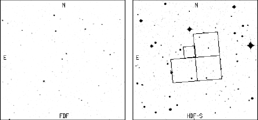	Figure 1: DSS plots of the FDF and of a field of the same size surrounding the HDF-S. Also indicated are the field boundaries of the HDF-S. Note the much lower surface density of bright foreground objects and the absence of bright stars in the FDF region.
Open with DEXTER

Following the pioneering work of Tyson (1988) several ground-based deep fields with a wide range of scientific drivers, sizes, limiting magnitudes and resolutions have been initiated. Examples are the NTT SUSI Deep Field (NTTDF, Arnouts et al. 1996), which has a size similar to the HDFs and sub-arcsecond resolution, but is a few magnitudes less deep than the HDFs, or the William Herschel Deep Field (WHTDF, Metcalfe et al. 2001 and references therein), which has a much larger field of view, a depth comparable to the HDFs, but lacks sub-arcsecond resolution. Other surveys, such as the Calar Alto Deep Imaging Survey (CADIS, Meisenheimer et al. 1998), are much shallower, but cover much larger areas (several 100 sq. arcmin in the case of CADIS ) and are specifically designed to search for primeval galaxies in the redshift range z = 4.6 - 6.7.

The aim of the FORS Deep Field (FDF) is to merge some of the strengths of the deep field studies cited above. The FDF programme has been carried out with the ESO VLT and the FORS instruments (Appenzeller et al. 1998) at a site, that offers excellent seeing conditions and allows imaging to almost the depths of the HDFs. The larger field of view compared to the HDFs (about 4 times the combined HDFs) alleviates the problem of the large-scale structure and results in larger samples of interesting objects. Moreover, spectroscopic follow-up studies with FORS can make full use of the entire field. Using the FORS2 MXU-facility, up to $\sim$60 spectra of galaxies (within 40 slitlets) in the FDF can be taken simultaneously.

In the present paper, the field selection of the FDF, the photometric observations and the data reduction are described. The first results have been described in Jäger et al. (1999). A source catalog (available electronically) based on objects detected in the B and I bands and containing 8753 objects in the FDF is described and its properties are discussed. This catalog supersedes a preliminary I-band selected catalog, which had been discussed by Heidt et al. (2000). Photometric redshifts obtained from the FDF will be discussed by Gabasch et al. (in prep.; see Bender et al. 2001 for preliminary results). Spectroscopic follow-up observations of a subsample of the FDF galaxies have been started. Up to now, spectra of about 500 galaxies with redshifts up to $z \sim 5$ have been analyzed. Initial results have been described in Appenzeller et al. (2002), Mehlert et al. (2001, 2002), Noll et al. (2001) and Ziegler et al. (2002).

2 Field selection

A critical aspect for a deep field study is the selection of a suitable sky area. Since we intended to obtain a representative deep cosmological probe of the Universe, one condition was that the galaxy number counts were not disturbed by a galaxy cluster in the field. To go as deep as possible also requires low galactic extinction ( E(B-V) < 0.02 mag). For the same reason, the field had to be devoid of strong radio or X-ray sources (potentially indicating the presence of galaxy clusters at medium redshifts). On the other hand, we decided to include a high-redshift (z > 3) radio-quiet QSO to study the IGM along the line-of-sight to the QSO and the QSO environment. To facilitate the observations in other wavebands, low HI column density (< $2 \times 10 ^{20}~ {\rm cm}^{-2}$) and low FIR cirrus emission was required. Moreover, stars brighter than 18th mag had to be absent to allow reasonably long exposures, to avoid saturation of the CCD and to minimize readout time losses. Because of the latter conditions, the HDF-S region was not suitable for our study (see Fig. 1). Additionally, stars brighter than 5th mag within $5\hbox{$^\circ$ }$ of the field had to be absent to avoid possible reflexes and stray-light from the telescope structure. Finally, the field had to have a good observability and, therefore, had to pass close to the zenith at the VLT site.

 

 

Table 1: Characteristics of the FORS Deep Field.

Field center	$1^{\rm h}6^{\rm m}3\hbox{$.\!\!^{\rm s}$ }6\ \ -25\hbox{$^\circ$ }45\hbox{$^\prime$ }46\hbox{$^{\prime\prime}$ }$ (2000)
mean E(B-V)	0.018
H I column density	$1.92 \times 10^{20}~ {\rm cm}^{-2}$
Radio sources (NVSS)	none with flux > 2.5 mJy
${\rm IRAS Cirrus}~ (100~ \mu{\rm m})$	0.035 Jy
Bright stars (<5 mag)	none within $5\hbox{$^\circ$ }$

 

 

Table 2: Observing log of the FDF observations.

Tel./Inst.	Dates	Filters	Comments
FORS1/UT1	Aug. 13-17 1999	g, R	mostly non-phot.
FORS1/UT1	Oct. 6-13 1999	U, B, g, R, I	during 3 nights
FORS1/UT1	Nov. 3-6 1999	U, B, R, I	3 $\times$ 0.5 nights
FORS1/UT1	Dec. 2-6 1999	U, B, R, I	4 $\times$ 0.3 nights
FORS1/UT1	July/Aug. 2000	B, I	3.5 hours each
SofI/NTT	Oct. 25-28 1999	J, Ks

Due to these constraints, the south galactic pole region was searched for a suitable field. We started by selecting all the QSOs from the catalog of Véron-Cetty & Véron (7th edition, 1997) with z > 3 within $10^{\circ}$ of the south galactic pole. This resulted in 32 possible field candidates. Next we did an extensive search in the literature from radio up to the X-ray regime (FIRST, IRAS maps, RASS etc.), checked visually the digitized sky survey and used the photometry provided by the COSMOS scans to select 4 promising field candidates containing a z > 3 QSO. For these 4 field candidates short test observations were carried out during the commissioning phase of FORS1, which showed that 3 of them were not useful (they either contained conspicuous galaxy clusters or, in one case, did not provide suitable guide stars for the active optics of the VLT). Finally, a field with the center coordinates $\alpha_{2000} = 1^{\rm h} 6^{\rm m} 3\hbox{$.\!\!^{\rm s}$ }6, \delta_{2000} = -25\hbox{$^\circ$ }45\hbox{$^\prime$ }46\hbox{$^{\prime\prime}$ }$ containing the QSO Q 0103-260 (z = 3.36, Warren et al. 1991) was chosen as the FDF. The characteristics of this field are summarized in Table 1. The Digital Sky Survey (DSS) prints in Fig. 1 provides a comparison of the FDF and the HDF-S, showing the great advantage of the FDF in relation to the HDF-S concerning the presence of bright stars.

3 Observations

Photometric observations using Bessel UBRI and Gunn g broad band filters were carried out with FORS1 at the ESO-VLT UT1 during 5 observing runs in visitor mode between August and December 1999. The data were complemented with some additional service-mode observations in the Bessel B and I filters with the same telescope in July and August 2000. Observing conditions were mostly photometric except for the August 1999 run, which was hampered by the presence of clouds and strong winds during some of the nights. In all cases a $2 \times 2$ k TEK CCD in standard resolution mode ( $0\hbox{$.\!\!^{\prime\prime}$ }2$/pixel, FOV $6\farcm8 \times 6\farcm8$), low gain and 4-port readout was used. The Gunn g filter was chosen instead of Bessel V in order to avoid the 5577 Å night sky emission line, thus reducing the background significantly.

From the field-selection images taken with FORS1 it was known that twilight flatfields alone are not sufficient for a data reduction reaching very faint magnitudes. Therefore the images were taken in a jittered mode. A 4 $\times$ 4 grid with a spacing of $8\hbox{$^{\prime\prime}$ }$was adopted in order to maximize the use of the scientific images for flatfielding purposes on the one hand, and to minimize the loss of field-of-view on the other hand. The order of the individual observing positions was such that images with the largest separation were always taken first.

Exposure times for the individual frames were set to 1200 s in U, 515 s in B and g, 240 s in R and 300 s in I. The seeing limit was initially set to $0\hbox{$.\!\!^{\prime\prime}$ }5$ for B and Iand $0\hbox{$.\!\!^{\prime\prime}$ }8$ for the remaining filters. Unfortunately, it became clear after the first observing run that those seeing limits were too strict (mainly due to the La Niña phenomenon at that period (Sarazin & Navarrete 1999; Sarazin 2000), and could not be met within a reasonable amount of telescope time. Therefore the seeing limits were relaxed to 1 $\hbox{$^{\prime\prime}$ }$ for U and g and $0\hbox{$.\!\!^{\prime\prime}$ }8$ for the B filter.

Due to the different seeing goals for each filter and varying seeing conditions during some of the nights, images in 3-5 filters were typically taken during each observing run. This resulted in somewhat longer exposure times on the summed images than initially anticipated (see Sect. 5). Photometric standards from Landolt (1992) were taken at least once during each photometric night.

NIR observations of the FDF in the J and Ks filter bands were acquired using SofI at the ESO NTT during 3 photometric nights in October 1999. Since the field-of-view of SofI with the large field objective is $4\farcm94 \times 4\farcm94$ ( $0\hbox{$.\!\!^{\prime\prime}$ }292$/pixel) only and, thus, significantly smaller than the field-of-view offered by FORS1, the observations were split into 4 subsets to cover the entire FDF.

In order to have as similar observing conditions as possible for all subsets, the observations in both NIR filters were distributed evenly over the three nights. Always at least all four subsets were observed subsequently in one filter for 20 min. Each set of 20 min consisted of 20 exposures of $10\times 6$ s. The positions of the four subsets were chosen so as to cover the entire FDF as observed by FORS with a maximal overlap of the subsets, but to avoid the southernmost 100 pixels of the SofI camera, which show image degradation (see SofI manual). To allow a good sky subtraction, jittered images were taken. We used a random walk jitter pattern within a rectangular box of $22\hbox{$^{\prime\prime}$ }$ border length centered on the central position of each subset. Photometric standard stars from Persson et al. (1998) were observed 3 times during each night to set the zero point.

In the end, the entire FDF was imaged effectively for 100 min in the two NIR filters. Due to the overlap of the individual subsets a narrow region was observed effectively for 200 min and the central region (including the QSO) effectively for 400 min. An overview of the optical and NIR observing runs and the filters used is given in Table 2.

4 Data reduction

Since we intended to reach with our FDF observations magnitude limits well below those of earlier ground-based studies, dedicated data reduction procedures had to be developed. On the other hand, the first spectroscopic follow-up observations of FDF galaxies were to start a few months after the last photometric observations of the FDF. In order to have candidate galaxies available at that time, a preliminary reduction of the photometric data taken in visitor mode was made and an I-band selected catalog with photometric redshifts was created. The content of this preliminary catalog has been described by Heidt et al. (2000), the photometric redshifts for this catalog by Bender et al. (2001).

In a second step, all data including the photometric data taken in service mode were reduced as described below. This data set forms the basis for the final photometric catalog described in the present paper.

   
4.1 Optical data

Because of the time variations of the CCD characteristics and of the telescope mirror (dust accumulation) each individual run was reduced separately. However, in order to have a data set as homogeneous as possible, the data reduction strategy was identical for all 5 runs.

Firstly, the images were corrected for the bias. Since the observations were done in 4-port readout mode, each port had to be treated separately. A masterbias was formed for each port by the scaled median of typically 20 bias frames taken during each run, and subtracted from the images scaling the bias level with the overscan.

Next the images were corrected for the pixel-to-pixel variations and large-scale sensitivity gradients. Since the twilight flatfields did not properly correct the large-scale gradients, a combination of the twilight flatfields and the science frames themselves was used. The twilight flatfields taken in the morning and evening generally differed considerably, and the twilight flatfields always left large-scale gradients on the reduced science frames (probably as a result of stray-light effects in the telescope and the strong gradient of the sky background at the beginning and the end of the night). Therefore, for each science frame, the sequence of flatfields was determined, which minimized the large-scale gradient. These sequences were normalized, median filtered and used for 1st order correction of the pixel-to-pixel variations. Typically 2-3 flatfields per filter per run had to be created this way, leaving residuals of the order of 2-8% (peak-to-peak) depending on the filter. To remove the residuals, the twilight-flatfielded science frames were grouped according to similar 2-dim large-scale residuals, normalized and stacked, using a 1.8 $\sigma$ clipped median. Afterwards a correction frame was formed by a 2-dim 2nd order polynomial fit to each median frame. This was done on a rectangular grid of $50 \times 50$ points, where the level of each grid point was taken as the median of a box with a width of 40 pixels. In this way it was guaranteed that no residuals from stars affected the fit and a noise free correction frame was achieved. Finally, each science frame was corrected for the pixel-to-pixel variations by a combination of the corresponding twilight flatfield and noise free correction frame. The peak-to-peak residuals on the finally reduced science frames were typically 0.2% or less.

Cosmic ray events were detected by fitting a two-dimensional Gaussian to each local maximum in the frame. All signals with a FWHM smaller than 1.5 pixels and an amplitude >8 times the background noise were removed. Then these pixels were replaced by the mean value of the surrounding pixels. This provides a very reliable identification and cleaning of cosmic ray events (for details see Gössl & Riffeser 2002).

In order to eliminate bad pixels and other affected regions for the image combination procedure, a bad pixel mask was created for every image. The positions of bad pixels on the CCD were determined for each filter for each run using normalized flatfields. All pixels whose flatfield correction exceeded 20% were flagged. Afterwards, each science frame was inspected for other disturbed regions (satellite trails, border effects) and their positions included in the corresponding bad pixel masks.

The alignment of the images and the correction for the field distortion was done simultaneously. This ensured a minimization of smoothing and S/N reduction. As a reference frame, an I filter image of the FDF taken under the best seeing conditions in October 1999 was used. Depending on the filter, the positions of 15-25 reference stars were measured via a PSF fit on each frame. A linear coordinate transformation was then calculated to project the images with respect to the reference image. The transformation included a rotation, a translation and a global scale variation. Finally, the correction for the field distortion was applied. Following the ESO FORS Manual, Version 2.4, we derive the FORS1 distortion corrected coordinates (x',y') in pixel units as a function of the distorted coordinates (x,y):

 

             x' = x-f(r)(x-x₀), (1)

y' = y-f(r)(y-y₀), (2)

where (x₀,y₀) are the coordinates of the reference pixel, $r=\sqrt{(x-x_0)^2+(y-y_0)^2}$ and

$$f(r)=3.602\times10^{-4}-1.228\times10^{-4}~r+2.091\times10^{-9}~r^2.$$ (3)

The flux interpolation for non-integer coordinate shifts was calculated from a 16-parameter, 3rd-order polynomial interpolation using 16 pixel base points (for details see Riffeser et al. 2001). The same shifting procedure was applied to the corresponding bad pixel masks, flagging as "bad" every pixel affected by bad pixels in the interpolation.

The images were then co-added according to the following procedure: First, the sky value of each frame was derived via its mode and subtracted. Then the seeing on each frame was measured using 10 stars, and the flux of a non-saturated reference star was determined. Next we assigned a weight to each image relative to the first image in each filter according to:

$$weight(n) = {\frac{f(n)}{f(1)}} \times {\frac{h(1 )\ {\it FWHM}(1)^2}{h(n)\ {\it FWHM}(n)^2}}$$ (4)

where n is the frame to be weighted relative to the 1st frame (1), f the flux of the reference star, h the sky level and FWHM the seeing on the frame. Weights computed according to Eq. (4) maximize the signal-to-noise ratio of the combined image for faint ( $f\ll h\times{\it FWHM}^2$) point sources. These are the overwhelming majority of the objects studied here. Finally, the weighted sum was calculated and normalized to a 1 s exposure time. Pixels flagged as bad on the individual images were not included in the coadding procedure. Since a different number of dithered frames contributed to each pixel in the co-added images, producing a position-dependent noise pattern, a combined weight map to each frame was constructed. The latter was included into the source detection and photometry procedure using SExtractor (see Sect. 6).

The photometric calibration of our co-added frames was done via "reference'' standard stars in the FDF. We first determined the zero points for two photometric nights (Oct. 10/11 and 11/12, 1999) during which the FDF was imaged in all 5 optical filters. The colour correction and extinction coefficients on the ESO Web-page were used to derive the zero points for our FORS filter set in the Vega system. As no calibration images were available in the g-band, transformation from V to g was performed following Jørgensen (1994). We then convolved all the FDF images from the two photometric nights to the same seeing as the co-added frames and determined the magnitudes of 2 (U)-10 (I) stars. Based on a curve of growth for these stars, a fixed aperture with a diameter of $8\hbox{$^{\prime\prime}$ }$ was used. Using these reference stars, we finally determined the zero points of the co-added frames. The difference of the magnitudes between the reference stars on the individual frames on the two photometric nights and on the co-added frames is 0.01 mag or less. We verified our zero points by repeating the procedure described above using observations from two photometric nights during our November 1999 run.

4.2 NIR data

About $\sim$10-20% of the observed NIR frames were found to contain an electronic pattern caused by the fast motion of the telescope near the zenith. These frames were excluded from the analysis. The remaining data were reduced using standard image processing algorithms implemented within IRAF. After dark-subtraction, for each frame a sky frame was constructed typically from the 10 subsequent frames which were scaled to have the same median counts. These frames were then median-combined using clipping (to suppress fainter sources and otherwise deviant pixels) to produce a sky frame. The sky frame was scaled to the median counts of each image before subtraction to account for variations of sky brightness on short time-scales. The sky-subtracted images were cleaned of bad-pixel defects and flat-fielded using dome flats to remove detector pixel-to-pixel variations. The frames were then registered to high accuracy, using the brightest $\sim$10 objects following the same procedure as described in the previous section, and finally co-added, after being scaled to airmass zero and an exposure time of 1 s.

The additionally observed photometric standard stars were used to measure the photometric zero point. The typical formal uncertainties in the zero-points were 0.02 mag in J and 0.01 mag in Ks.

5 Basic properties of the co-added images

A summary of the properties of the individual co-added images is presented in Table 3. The total integration time for the co-added images is given as well as the number of frames used, the average FWHM measured on 10 stars across the field, the area with 80% weight for each individual image and the 50$\%$ completeness limits for a point source as described in Sect. 6.

 

 

Table 3: Overview of the photometric observations.

Band	Exposure	Frames	FWHM	80% weight	50$\%$ compl. limit
	Time [s]		[ $^{\prime\prime}$]	[ $\hbox{$^\prime$ }^2$]	[mag]
U	44 400	37	0.97	40.7	25.64
B	22 660	44	0.60	40.5	27.69
g	22 145	43	0.87	41.1	26.86
R	26 400	110	0.75	40.8	26.68
I	24 900	83	0.53	40.9	26.37
J	$4800^{\rm a}$	$80^{\rm a}$	1.20	4.2/53.8	23.60/22.85
Ks	$4800^{\rm a}$	$80^{\rm a}$	1.24	4.4/53.7	21.57/20.73

$^{\rm a}$ Minimum exposure time and number of frames for each subset. Due to the overlap of the subsets for some (small)
regions of the FDF the total time was twice or even four times this value. The 80% weight and 50% completeness
levels in J and Ks are given for the 320 (central field) and 80-minutes co-added data, respectively.

The integration times are in total almost a factor of 2 higher than originally planned (except for the U filter). This is due to our strict seeing limits during the first observing runs. It compensates, at least in part, the loss of resolution/depth of the images due to the less than optimal seeing. Still, the completeness limits are somewhat lower than expected for the integration times since the efficiencies of the telescope (reflectivity of the main mirror) and the CCD were below expected at the time of the observations. In general, the zero points remained relatively constant during the observations carried out in 1999, whereas they differed considerably between the observations taken in 1999 and 2000. This resulted in a loss of approx. 0.3 mag (see the ESO-Web page, Paranal zero points).

The area with 80% weight is very similar for all optical bands and 30% larger for the NIR bands. The latter is due to the 4 subsets taken during the NIR observations. The common area with 80% weight in all filters is $39\farcm8^2$.

As an example, the co-added I band image of the FDF is displayed in Fig. 2. The common area of the input images for a $6\hbox {$^\prime $ }\times 6\hbox {$^\prime $ }$ region is shown here. It contains $\sim$6100 galaxies. In general, the galaxies are distributed evenly across the field. There is a poor galaxy cluster (at $z \sim 0.3$) in the southwestern corner of the FDF. The QSO Q 0103-260 is south of the center of the frame and is marked with an arrow. The brightest object in the field is an elliptical galaxy with ${m}_{\rm I} = 16.5$ at $z \sim 0.2$ in the southeastern part of the FDF.

6 Source detection and photometry

We used SExtractor (Bertin & Arnouts 1996) with the WEIGHT-IMAGE-option and WEIGHT-TYPE = MAP-WEIGHT for the source detection and extraction on the images. The weight-maps described above were used to account for the spatial dependent noise pattern in the co-added images, and in particular to pass the local noise level of the data to the SExtractor program.

Figure 2: The FDF in I band from FORS observations. The common area of all input frames for a field of view of $6\hbox {$^\prime $ }\times 6\hbox {$^\prime $ }$ is shown here. North is up, east to the left. The total integration time was 6.9 h, mean ${\it FWHM} \sim 0\hbox{$.\!\!^{\prime\prime}$ }53$. The QSO Q 0103-260 is south of the center of the frame and marked with an arrow. This area contains $\sim$6100 galaxies. Note the even distribution of galaxies across the frame, except for the small galaxy concentration in the southwestern corner. The brightest object in the field is the large elliptical galaxy in the southeastern part of the FDF at $z \sim 0.2$ with ${m}_{\rm I} = 16.5$.

Open with DEXTER

To use SExtractor, three parameters have to be set: i) The detection threshold t, which is the minimum signal-to-noise ratio of a pixel to be regarded as a detection, ii) the number n of contiguous pixels exceeding this threshold, iii) the filtering of the data prior to detection (e.g. with a top-hat or a Gaussian filter). We used a Gaussian filter with a width $\theta_F$, for the $\theta_F$ values see below.

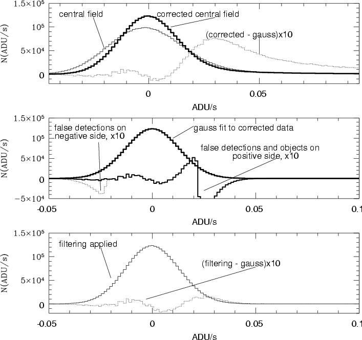Figure 3: Pixel-value histograms (in ADU per second) for the (central field) I image at various analysis stages. Upper panel: histogram of the original data (thin line) and after subtracting the low frequency spatial variations due to the non-uniform sky background (thick line). Also included is the difference of the corrected histogram and a Gaussian (shown as thick line in the middle panel) fitted to its negative (ADU/s < 0) wing. This negative wing should not be affected by real objects and therefore should represent the true noise in the image. For clarity the difference has been scaled up by a factor of 10 and the curve has been labeled accordingly. The real objects show up as a positive excess of the pixel values in the corrected data distribution and in the difference function at positive ADU/s. Middle panel: the thick line shows the Gaussian derived by fitting the negative wing of the corrected data distribution as described above. Its difference to the pixel-value distribution derived for those pixels where SExtractor (with optimal parameters but without filtering) finds no objects (or object contributions) is shown as a solid line. The corresponding difference distribution of the inverted image is shown dotted for the negative ADU/s only. The negative excess shows the false detections due to the correlated error. The difference curves are again scaled up by a factor of 10. Lower panel: the thin line shows the histogram of the pixel values of pixels not belonging to objects when SExtractor is run after filtering the corrected data with a (2 pixel FWHM) Gaussian. The dotted line shows the difference between this histogram and the Gaussian fit shown in the middle panel. The number of significant false detections has now dropped to nearly zero.

Open with DEXTER

We varied these parameters to maximize the number of source detections, while minimizing false detections. The following procedure, described here for the I-band data, was used for all filters. We first considered only those pixels in the field where the exposure time equaled the total exposure time (the weight-map took care of the correct scaling of RMS for the full field later on) and called this part of data the "central field".

If there were no objects in the field and if the data reduction resulted in a perfectly flat sky we would expect the histogram of the pixel-values to be a Gaussian, with a width reflecting the photon-noise and the correlated noise of the data reduction and coaddition procedure. The actual histogram of pixel-values of the central-field is shown in Fig. 3 (upper panel, thin line). Even ignoring the wings, the histogram is asymmetric around its center at zero. This stems from the non-uniformities of the sky background, that amount to about 1% (see Sect. 4.1). Therefore, we determined the sky-curvature on large scales and subtracted a 2-dimensional fit to this surface from the original data. The corrected histogram of pixel-values (Fig. 3, upper panel, thick curve) is now symmetric around its center at zero and the left-hand part is well described by a Gaussian (with a width of 0.01295 ADU/s). The right hand part shows an excess above $\approx$0.015 ADU/s, which is due to the objects in the field (see difference curve in Fig. 3, scaled up by a factor 10). We have checked that it does not make any difference for the detection and the photometry of reliable objects whether the procedure is applied to the original or to the corrected data: for each object, the difference between the magnitude estimates of these two cases is smaller than the assigned magnitude RMS-error. This implies that we can carry out the adjustment of optimum SExtractor parameters in the corrected version of the data.

To optimize the pre-detection filtering procedure we made the following numerical experiment. We generated a "negative version'' of an image by multiplying it by -1 and a "randomized version'' by randomly assigning measured pixel values to new positions (the weights of the weight-map are re-localized the same way). With no filtering ( $\theta_F=0$) and using t = 1.7 and n = 3 SExtractor finds about 9000 objects in the original image, 5600 in the negative one and 1100 in the randomized one. The fact that many more objects are detected in the negative image than in the randomized one indicates that correlated noise is present in both the negative and the positive images. Therefore filtering must be used to specifically suppress the small-scale noise. It is possible that large-scale noise is still present, but there is no way to remove such a component. By varying the width $\theta_F$ of a Gaussian filter we found that $\theta_F = 2$ is an optimal choice. With n=3 and t=1.7 the number of objects detected on the negative image dropped to the expected random number, nearly zero. Of course, once $\theta_F$ is fixed, one is still left with the freedom of trading n for t by increasing the number of pixels above the threshold and decreasing the threshold value at the same time. We decided to keep n small, in order to obtain an unbiased detection of faint point sources. This choice allows us to exploit the excellent seeing of the I-band data, where the FWHM is only 2.5 pixels.

Now we illustrate our procedure more quantitatively: we ran SExtractor (for each choice of $\theta_F$, n and t) on the positive, the negative and the randomized images. We registered all pixels which were covered by objects, removed them from the pixel-value statistics and normalized the corresponding pixel-value histogram to the total number of pixels in the central field, and we call that the "background-histogram''. We expect that for good source extraction parameters, the background histograms will look like a Gaussian, more precisely like that Gaussian derived by fitting the negative wing of the corrected data distribution, which we call the "optimum-background-histogram'' below. The difference (magnified by a factor of 10) to that optimum background histogram is shown in the middle panel of Fig. 3 for n=3, t = 1.7, $\theta_F=0$ for detection on the positive (solid) and negative (dotted, for negative ADU/s only) image. The negative excess of these histograms below zero are false detections due to correlated noise. Increasing $\theta_F$ these false detections drop dramatically when $\theta_F = 2$ pixels is reached. Then, n=3 and t=1.7 were fixed by requiring no false detections on the negative image, i.e. no detections due to correlated noise. We finally run SExtractor with this set of parameters on the positive image, obtain the background histogram and show the difference to the optimum background histogram in the lower panel of Fig. 3 (dotted histogram, magnified by a factor of 10). The difference is indeed very small.

Using the above parameters ( $\theta_F = 2$ with a Gaussian convolution, n=3 and t = 1.7), obtained from the optimum pre-detection filtering and the requirement of no-detection on the negative image, we find that the extended wing in the ADU-histogram due to the presence of objects disappears and that the histogram becomes symmetrical and Gaussian (see Fig. 3, bottom panel). This demonstrates that with this choice of parameters we are optimally extracting all objects above the noise level, without getting significant false detections. The adopted parameters give a (total) photometric accuracy better than 5$\sigma$.

The optimum parameters were finally used to run SExtractor on the (positive and negative) images of the total FDF. We found about 6900 objects on the positive and less than a handful of objects on the negative side of the entire I image. All these spurious detections occurred near discontinuities of the S/N level outside the central field and were caused by the non perfectly flat sky, which makes some of the discontinuities more pronounced than they should be according to the photon-noise and the corresponding weight-map.

The same analysis described for the I-band image was carried out for the other filters. We emphasize here that our extraction procedure was optimized to maximize the number of real detections for a reliable photometry and hence reliable photometric redshifts rather than to study galaxy number counts at the faintest limits. For the optical bands, we used the same extraction parameters. For the NIR-data we opted for $\theta_F=3$ pixels to match the pixel size of the original NIR-data, which is roughly 1.5 the pixel size of FORS, and t=2.0 and n=5 for the J band, and t=1.9 and n=5for the Ks band, to take into account the poorer seeing and the different noise level. To illustrate the reliability of our detection procedure we display a detection file returned from SExtractor for a $1\hbox {$^\prime $ }\times 1\hbox {$^\prime $ }$ region of the northern part of the FDF in Fig. 4.

The photometric errors presented in the final catalog are those derived by the SExtractor routine. To make sure that the error calculation was not influenced by correlated noise in the sky background, the results of the SExtractor were verified with aperture photometry with different apertures in areas not covered by objects and by estimating the expected photometric errors from the background variations. In general we found good agreement with the SExtractor derived errors. In particular the SExtractor errors were found to be quite accurate for point sources and for small objects. Only in the case of large extended objects may non-stochastic background variations have resulted in an underestimate of the photometric errors. But the few objects possibly affected are normally bright and have small errors, which should still be correct within the numbers given in the catalog.

Finally, we calculated the 50% completeness levels in each filter band using our extraction parameters and the formula given in Snigula et al. (2002). This approach estimates the completeness limit by calculating the brightness at which the area of pixels brighter than the applied flux limit falls below the size threshold of the detection algorithm (for a given FWHM of a point source). To allow a comparison with other deep fields, the data were corrected for galactic extinction as described in Sect. 7. The results are summarized in Table 3.

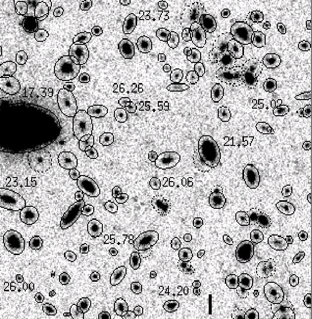Figure 4: Detection file returned from SExtractor for a $1\hbox {$^\prime $ }\times 1\hbox {$^\prime $ }$ region of the northern part of the FDF. It illustrates the reliability of our detection and photometry procedure. The I-band image shown here contains $\sim$160 objects. For some objects the integrated magnitudes are displayed. The detection file shows the elliptical aperture limits used to derive mag_auto. Dashed ellipses denote blended objects.

Open with DEXTER

7 Photometric catalog

7.1 Compilation of the photometric catalog

To create the final photometric catalog we merged the individual catalogs of the objects detected in the co-added B filter image and in the co-added I filter image. We decided to use these two catalogs as a basis, since the images in these two filters correspond to the best seeing conditions and since most types of objects are expected to be detected in at least one of these two bands.

The merging of the I and B catalogs was carried out as follows: we first matched the positions of the detected objects and their corresponding images in the two filters. This was done by visual inspection of the entries of the objects on both frames. This procedure gave us a clear view of the success of our automatic detection procedure and allowed us to reject obviously false identifications. In order to avoid mis-matches in the final catalog, each entry in the B catalog was first assigned a corresponding entry in the I catalog and vice versa. A cross-match of the B versus I and I versus B entries allowed us to identify false matches, which were checked again until a perfect cross-match was derived.

The initial catalogs in B and I contained 7206 and 6900 entries, respectively. After the visual cross-matching, we deleted 15 objects from the B catalog and 8 objects from the I catalog. These were mostly objects close to the edges of the field. In a few cases, 2 objects separated by a few pixels (e.g. a merging pair of galaxies) were detected in the B band, whereas in the I band only one object in between the two B band objects was found (essentially at the center of the common envelope of both galaxies). In such cases the entry in the I band was deleted. This left us with 7191 entries in the B catalog and 6892 entries in the I catalog. Now we merged both catalogs to form the final photometric catalog. This catalog contains 8753 objects. 5327 out of the 8753 objects were detected in both filters (61%), whereas 1864 (21%) were detected in B only and 1562 (18%) were detected in I only. We emphasize here that a non-detection does not necessarily mean that the object is not present on the frame, it rather means that the object was not detected by SExtractor with the parameters set here.

Since SExtractor may use a different number of pixels to derive the total magnitudes in B and I, the colours of very extended objects computed from the total magnitudes are not reliable. Therefore the catalog also contains aperture magnitudes in UBgRIJKs. An aperture of $2\hbox{$^{\prime\prime}$ }$ was chosen in order to minimize the errors due to blending and since the faint objects usually have diameters of $\leq 2\hbox{$^{\prime\prime}$ }$. The aperture magnitudes were derived by first convolving all frames to the same seeing ( $1\hbox{$^{\prime\prime}$ }$ FWHM) and then performing aperture photometry on the positions of the objects detected in B and I in the convolved frames. For objects detected in B only, we used the aperture photometry based on the positions in the B catalog, whereas the aperture photometry based on the positions in the I catalog were used for the remaining objects (detection on both frames or I-only detections). Thus for many objects, which were initially not detected in either filter, useful photometric data could be given.

Finally, the galactic absorption towards the FORS Deep Field was estimated. We used the formulae 2 and 3 in Cardelli et al. (1989) and adopted E(B-V) = 0.018 (Burstein & Heiles 1982) and $A_V = 3.1 \times {E}({B}-{V})$ to calculate the extinction correction for each filter. The central wavelengths for each filter were taken from the ESO Web-page. We derived A_U/A_V = 1.555, A_B/A_V = 1.365, A_g/A_V = 1.105, A_R/A_V = 0.790, A_I/A_V = 0.631, A_J/A_V = 0.283 and A_Ks/A_V = 0.117resulting in A_U = 0.087 mag, A_B = 0.076 mag, A_g = 0.062 mag, A_R = 0.041 mag, A_I = 0.035 mag, A_J = 0.016 mag and A_Ks = 0.007 mag, respectively. The values for the extinction agree to $\leq$0.01 mag with those listed in the NED. The photometric catalog described below is not corrected for galactic extinction. However, the completeness limits as well as the number counts shown in Sect. 8 were derived with a galactic extinction correction.

7.2 Contents of the photometric catalog

The full catalog containing 8753 objects is available in electronic form at CDS via anonymous ftp to cdsarc.u-strasbg.fr (130.79.128.5) or via http://cdsweb.u-strasbg.fr/cgi-bin/qcat?J/A+A/398/49.

As an illustration of its content we list in Table 4 the entries 2630-2639.

For each object we report the following parameters:

ID: the identification number. The objects have been sorted first by right ascension (2000), followed by declination (2000). The identification numbers provide a cross-reference to the spectroscopic and other observations of the FDF (e.g. Noll et al., in prep.).

RA, Dec: the positions of the objects in the FDF for J2000.0. Their accuracy has been examined by comparing the positions of 31 well-isolated, evenly distributed objects on the I frame of the FDF, to those listed in the USNO catalog (Monet 1998). The mean difference in right ascension is $0\hbox{$.\!\!^{\prime\prime}$ }21\pm0\hbox{$.\!\!^{\prime\prime}$ }38$ and the mean difference in declination is $0\hbox{$.\!\!^{\prime\prime}$ }14\pm0\hbox{$.\!\!^{\prime\prime}$ }40$. Given a typical accuracy of $0\hbox{$.\!\!^{\prime\prime}$ }25$ for objects in the USNO catalog our positions have an accuracy of $\sim$ $0\hbox{$.\!\!^{\prime\prime}$ }5$.

${m}_{\rm BT}$, $\sigma_{\rm BT}$, ${m}_{\rm IT}$, $\sigma_{\rm IT}$: the total magnitudes (Vega-system) and associated mean errors of the detected sources in the B and I band images, respectively, as measured using the SExtractor routine mag_auto on the co-added and unconvolved frames. Mag_auto is an automatic aperture routine based on Kron's (1980) "first moment'' algorithm, which determines the sum of counts in an elliptical aperture. The semimajor axis of this aperture is defined by 2.5 times the first moments of the flux distribution within an ellipse roughly twice the isophotal radius, within a minimum semimajor axis of 3.5 pixels. This routine is intended to give the most precise estimate of "total magnitudes'', at least for galaxies, and takes into account the blending of nearby objects.

${m}_{\rm UBgRIJKs [2\hbox{$^{\prime\prime}$ }]}, \sigma_{UBgRIJKs}$: UBgRIJKs magnitudes (Vega-System) and associated errors within an aperture of $2\hbox{$^{\prime\prime}$ }$. They (and their errors) were measured on the co-added and convolved frames using SExtractor. The positions listed in the catalog were used for this procedure. An aperture of $2\hbox{$^{\prime\prime}$ }$ was chosen in order to minimize the errors due to blending. Moreover, the faint objects in the FDF usually have diameters of $\leq$2 $\hbox{$^{\prime\prime}$ }$. Choosing a larger aperture would result in larger photometric errors due to the sky background. For extended objects, the mean errors of the aperture magnitudes are generally smaller than for the total magnitudes, as the aperture photometry selected the regions of high surface brightness. The magnitudes were not corrected for blending. Blended objects can be identified from the column Flag1 (see below).

 

Table 4: Excerpt from the FDF object catalog. The entries with the IDs 2630-2639 are displayed as examples.

ID	RA (2000)	Dec (2000)	${m}_{\rm BT}$	$\sigma_{\rm BT}$	${m}_{\rm IT}$	$\sigma_{\rm IT}$	mU [ $2\hbox{$^{\prime\prime}$ }$]	$\sigma_{U}$	mB [ $2\hbox{$^{\prime\prime}$ }$]	$\sigma_{B}$	mg [ $2\hbox{$^{\prime\prime}$ }$]	$\sigma_{g}$	mR [ $2\hbox{$^{\prime\prime}$ }$]	$\sigma_{R}$	mI [ $2\hbox{$^{\prime\prime}$ }$]	$\sigma_{I}$
2630	1 5 57.28	-25 48 02.3	27.75	0.19	25.30	0.10	26.99	0.27	27.61	0.05	27.72	0.10	26.10	0.03	25.34	0.02
2631	1 5 57.29	-25 45 00.1			24.42	0.03					30.73	1.65	26.57	0.04	24.49	0.01
2632	1 5 57.29	-25 48 46.9	26.13	0.05	24.98	0.07	25.96	0.10	26.20	0.01	25.92	0.02	25.42	0.02	25.05	0.02
2633	1 5 57.30	-25 44 56.6	24.47	0.01	22.75	0.01	24.60	0.03	24.60	0.01	23.74	0.01	23.26	0.01	22.87	0.01
2634	1 5 57.30	-25 48 14.2	27.69	0.16					27.77	0.06	28.23	0.17	26.84	0.06	26.78	0.09
2635	1 5 57.31	-25 43 52.3			25.02	0.09	26.22	0.13	26.42	0.02	26.11	0.02	25.66	0.02	25.33	0.02
2636	1 5 57.31	-25 44 02.2	24.85	0.04	23.43	0.04	25.53	0.07	25.53	0.01	25.12	0.01	24.56	0.01	24.12	0.01
2637	1 5 57.31	-25 44 15.2	26.60	0.09	26.19	0.17	26.76	0.22	26.83	0.02	26.72	0.04	26.46	0.04	26.16	0.05
2638	1 5 57.31	-25 46 23.5	27.36	0.16	25.65	0.09	27.58	0.46	27.43	0.04	27.45	0.08	26.72	0.05	25.67	0.03
2639	1 5 57.31	-25 47 51.1	26.17	0.08	25.11	0.10	26.42	0.16	26.85	0.02	26.74	0.04	26.22	0.03	25.60	0.03

ID	mJ [ $2\hbox{$^{\prime\prime}$ }$]	$\sigma_{J}$	mKs [ $2\hbox{$^{\prime\prime}$ }$]	$\sigma_{Ks}$	FWHM [ $^{\prime\prime}$]	Elong	PA [$^\circ$]	Cstar	Flag1	Flag2	Flag3	weight_B	weight_I
2630			21.97	0.20	0.74	1.17	17.9	0.40	0			1.000	1.000
2631	21.36	0.01	20.35	0.03	0.52	1.02	111.7	0.98	0	Ionly	L star		1.000
2632	26.58	2.38	22.37	0.29	0.78	1.12	82.1	0.26	0			1.000	1.000
2633	22.09	0.03	20.91	0.06	0.53	1.04	36.2	0.98	0		QSO	1.000	1.000
2634					1.01	1.25	00.6	0.61	0	Bonly		1.000
2635	23.70	0.18			1.13	1.19	129.3	0.00	3	Ionly			0.984
2636	22.71	0.07	20.75	0.07	0.73	1.34	90.2	0.09	3			0.984	1.000
2637					1.07	1.87	76.9	0.40	0			1.000	1.000
2638					0.80	1.49	19.1	0.43	0			1.000	1.000
2639	24.02	0.23	22.96	0.50	1.34	1.16	21.6	0.01	2			1.000	1.000

The next four columns (FWHM, elongation, position angle, star-galaxy classification parameter) describe the morphology of the objects. Since the FWHM, elongation and position angle may have high errors and are sometimes unreliable for faint objects, this information is provided for objects brighter than our 50$\%$ completeness limit (27.69 in B, 26.37 in I) only. Moreover, we do not list these values for objects where SExtractor derived a ${\it FWHM} < 0\hbox{$.\!\!^{\prime\prime}$ }4$(FWHM is $0\hbox{$.\!\!^{\prime\prime}$ }53$ in co-added I band frame and $0\hbox{$.\!\!^{\prime\prime}$ }6$ in co-added B band frame). The information should also be treated with caution for brighter objects having a star-galaxy classification parameter >0.9.

FWHM: Full width at half maximum of the objects in arcsec as determined by SExtractor by a Gaussian fit to the core.

Elong: Elongation of the images. The elongation is defined as A/B, where A and B are given by the 2nd order moment of the light distribution along the major and minor axis, respectively.

PA: The position angle of the major axis, measured from North to East, with N-S = 0.

Cstar: Star-galaxy classification parameter returned by SExtractor based on the morphology of the objects on the image. A classification near 1.0 describes point like sources whereas a classification close to 0.0 describes extended sources.

Flag1: flags returned by SExtractor with the following notation:

1: object has neighbours bright and close enough to bias significantly mag_auto; 2: the object was originally blended with another one; 3: sum of 1 + 2; 4: at least one pixel of the object is saturated (or very close to saturation); 7: sum of 1 + 2 + 4; 8: the object is truncated (e.g. too close to the image boundary); 16: object aperture data are incomplete or corrupted; 17: sum of 1 + 16; 18: sum of 2 + 16; 19: sum of 1 + 2 + 16; 24: sum of 8 + 16.

Flag2: here we report if an object was detected on the B frame only ("Bonly''), on the I frame only ("Ionly''). If there is no entry, the object is detected by SExtractor on both frames.

Flag3: a preliminary classification of 35 point-like objects (QSOs, stars) from our spectroscopic survey (Noll et al., in prep.).

weight_B, weight_I: averaged weights of all pixels used to determine ${m}_{\rm BT}$ and ${m}_{\rm IT}$, respectively. They were derived from the combined weight maps which are described in Sect. 4. A weight of 1 means that all pixels used to derive the magnitude are fully exposed and not affected by bad areas. Most of the detections with low weights are close to the edges of the FDF where the total integration times are lower.

8 Galaxy number counts

The number counts serve as a quick check of the approximate photometric calibration and for the depth of the data. We did not put much effort in star-galaxy separation at the faint end, where the galaxies dominate the counts anyway. At the bright end, where SExtractor is able to disentangle a stellar and a galaxy profile, we derived limits by investigating the class-FWHM diagram for the objects. In the following figures, the counts for all objects are shown as dashed histograms, while for the solid line histograms obvious stellar objects have been omitted. The magnitudes are given in the Vega-system. The number counts are given only for the area with maximum integration-times (weight-map $\approx$1) for the optical data and for ${\rm weight-map} \ga 0.25$ for the NIR-data (i.e. we exclude the edges of the fields). They are not corrected for incompleteness. Also indicated is the 50% completeness limit for the detection of point sources. For each filter we also included for comparison number-magnitude-relations obtained in earlier observations which are compiled and transformed to standard filter systems in Metcalfe et al. (2001) for the optical filters. In all cases we plot raw number counts only, i.e. we do not correct for incompleteness at the faint end.

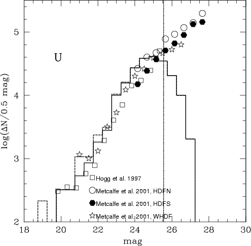	Figure 5: Galaxy number counts of the FDF in the U band (not corrected for incompleteness) as compared to other deep surveys. The vertical dash-dotted line indicates the 50% completeness limits.
Open with DEXTER

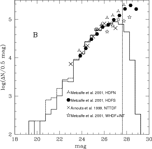	Figure 6: Galaxy number counts of the FDF in B band (not corrected for incompleteness) as compared to other deep surveys. The vertical dash-dotted line indicates the 50% completeness limits.
Open with DEXTER

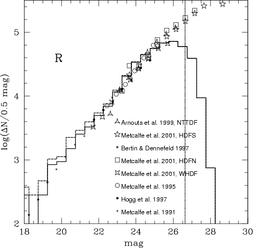	Figure 7: Galaxy number counts of the FDF in R band (not corrected for incompleteness) as compared to other deep surveys. The vertical dash-dotted line indicates the 50% completeness limits.
Open with DEXTER

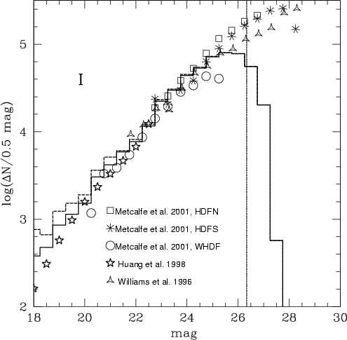	Figure 8: Galaxy number counts of the FDF in I band (not corrected for incompleteness) as compared to other deep surveys. The vertical dash-dotted line indicates the 50% completeness limits.
Open with DEXTER

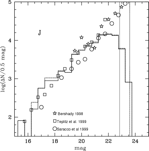	Figure 9: Galaxy number counts of the FDF in J band (not corrected for incompleteness) as compared to other deep surveys. The vertical solid line indicates the 50% completeness for the shallower exposed part of the field, whereas the vertical dash-dotted line indicates the 50% completeness for the deeply exposed part of the field.
Open with DEXTER

In the U-band the FDF is 50$\%$ complete to U = 25.64 mag for a point source. The slope agrees with earlier measurements (roughly 0.4-0.5) for U<23 and it becomes shallower (0.35 at U=23-25), in agreement with the slopes of the HDF-S, WHDF and Hogg et al. (1997) (see Metcalfe et al. 2001). In Fig. 5 we have transformed the HDF number counts as proposed by Metcalfe et al. using $F_{\rm 3oo,Vega}=U-0.4$ and Table 5 in their paper. We further assume $U_{\rm WHDF}\approx U$ to include the WHDF U-band-raw counts (Table 4 of Metcalfe et al. 2001) - in fact the central wavelengths and the transmission curves of the U filters used for the FDF and WHDF observations are similar. The values of Hogg et al. (1997) have been obtained from their Fig. 3 and been transformed as proposed by Metcalfe, $U\approx U_{\rm Hogg}+0.08$. The HDFN/S and WHDF number counts are not corrected for reddening (Metcalfe, private comm., $E(B-V)_{\rm WHDF}\approx 0.02$which is similar to the FDF and thus would shift the number counts by $\approx$-0.1).

Our B-band number counts (Fig. 6) are 50$\%$-complete at 27.69 mag. Within the field-to-field variations they agree well with the HDFS/N (we follow Metcalfe et al. (2001) and use the transformation $F_{450,\rm Vega} \approx B -0.1$) and the raw-counts in the NTT deep field (Arnouts et al. 1996). We also included the raw counts in the Herschel deep field, assuming $B_{\rm FDF}\approx B_{\rm WHDF}$.

For the g-band, we just show our results in Fig. 10 without comparison, since no adequate number counts have been presented in the literature for this passband. Our estimated 50% completeness limit is 26.86 mag in this filter.

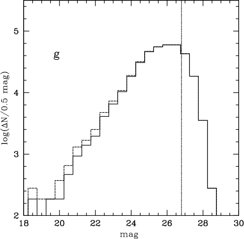	Figure 10: Galaxy number counts of the FDF in g band (not corrected for incompleteness). The vertical dash-dotted line indicates the 50% completeness limits.
Open with DEXTER

Our R-band and I-band data are $50\%$-complete at 26.68 mag and 26.37 mag, respectively. Amplitude and slope agree well with previously published fields. For the transformation of the HDF-counts we followed Metcalfe et al. 2001) and used $R\approx R_{606,\rm Vega}-0.1$ and $I\approx I_{814,\rm Vega}$; we also assumed that $R \approx R_{\rm WHDF}$. The counts are shown in Figs. 7 and 8.

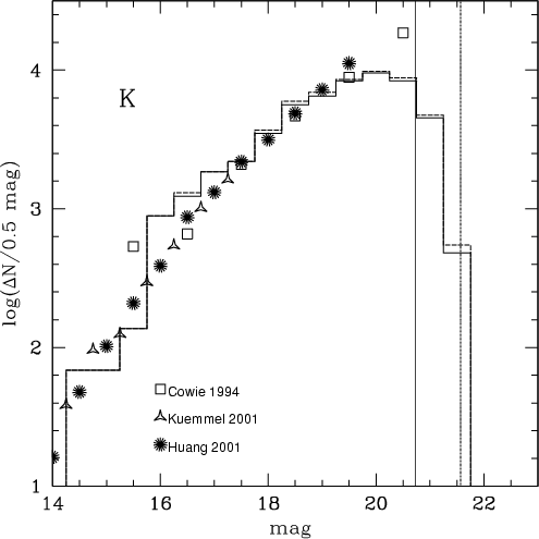	Figure 11: Galaxy number counts of the FDF in Ks band (not corrected for incompleteness) as compared to other deep surveys. The vertical solid line indicates the 50% completeness for the shallower exposed part of the field, whereas the vertical dash-dotted line indicates the 50% completeness for the deeply exposed part of the field.
Open with DEXTER

Our number counts in the J-band (Fig. 9) agree with those derived by Saracco et al. (1999), and precisely match those of Teplitz et al. (1999). The completeness is 22.85 mag and 23.60 mag for the shallower and deeply exposed (factor of four in integration time) part of the field, respectively. Our number counts in the K-band (Fig. 11) agree well with those of Kümmel & Wagner (2001) and Huang et al. (1998). The completeness limits are 20.73 mag and 21.57 mag for the shallow and deep exposed part of the field. For fairly shallow J and K pointings ($J\la 22$ and $K\la 20$) the field-to-field variations are expected to be significant for our field size, since the distribution of massive, old systems dominating the NIR frames varies considerably on small scales. This has been demonstrated e.g. in the different pointings of the MUNICS survey by Drory et al. (2001). The agreement with other surveys is good and the quoted detection limit correspond to the 50% completeness limit of our sample.

Acknowledgements

We thank the Paranal and NTT staff at ESO for their excellent and very efficient support at the telescope. We also thank the referee (Dr. M. Franx) for his constructive comments. This work has been supported by the Deutsche Forschungsgemeinschaft (SFB 375, SFB 439), the VW foundation (I/76520) and the German Federal Ministry of Science and Technology (Grants 05 2HD50A, 05 2GO20A and 05 2MU104).

We have made use of the Simbad Database, operated at CDS, Strasbourg, France, and the NASA/IPAC Extragalactic Database (NED), operated by the Jet Propulsion Laboratory, California institute of Technology under contract with the National Aeronautics and Space Administration.

References

 
• Appenzeller, I., Fricke, K., Fürtig, W., et al. 1998, The Messenger, 94, 1 In the text NASA ADS  
• Appenzeller, I., Mehlert, D., Noll, S., et al. 2002, High redshift galaxies in the FORS Deep Field; in Studies of Galaxies in the Young Universe with New Generation Telescopes, ed. N. Arimoto, ADS Electronic Publications 2002, in press In the text  
• Arnouts, S., D'Odorico, S., Cristiani, S., et al. 1999, A&A, 341, 641 In the text NASA ADS  
• Bender, R., Appenzeller, I., Böhm, A., et al. 2001, The FORS Deep Field: Photometric redshifts and object classification, in Deep Fields, ed. S. Cristiani, A. Renzini, & R. E. Williams, ESO astrophysics symposia (Springer), 96 In the text  
• Bershady, M. A., Lowenthal, J. D., Koo, D. C. 1998, ApJ, 505, 50 NASA ADS  
• Bertin, E., & Arnouts, S. 1996, A&AS, 117, 393 In the text NASA ADS  
• Bertin, E., & Dennefeld, M. 1997, A&A, 317, 43 NASA ADS  
• Burstein, D., Heiles, C. 1982, AJ, 87, 1165 In the text NASA ADS  
• Cardelli, J. A., Clayton, G. C., Mathis, J. S. 1989, ApJ, 345, 245 In the text NASA ADS  
• Cohen, J. G. 1998, Redshift clustering in the Hubble Deep Field; in The Hubble Deep Field, ed. M. Livio, S. M. Fall, & P. Madau, STScI Symposium Series, 11, 52 In the text  
• Connolly, A. J., Szalay, A. S., Dickinson, M., Subbaro, M. U., Brunner, R. J. 1977, ApJ, 486, L11 NASA ADS  
• Cowie, L. L., Gardner, J. P., Hu, E. M., et al. 1994, ApJ, 434, 114 NASA ADS  
• Drory, N., Feulner, G., Bender, R. 2001, MNRAS, 325, 550 In the text NASA ADS  
• Gössl, C. A., & Riffeser, A. 2002, A&A, 381, 1095 In the text NASA ADS  
• Heidt, J., Appenzeller, I., Bender, R., et al. 2000, Rev. Mod. Astr., 14, 209 In the text  
• Hogg, D. W., Pahre, M. A., McCarthy, J. K., et al. 1997, MNRAS, 288, 404 In the text NASA ADS  
• Huang, J.-S., Cowie, L. L., & Luppino, G. A. 1998, ApJ, 496, 31 In the text NASA ADS  
• Huang, J.-S., Thompson, D., Kümmel, M. W., et al. 2001, A&A, 370, 909 NASA ADS  
• Jørgensen, I. 1994, PASP, 106, 967 In the text NASA ADS  
• Kajisawa, M., & Yamada, T. 2001, PASJ, 53, 833 In the text NASA ADS  
• Kron, R. G. 1980, ApJS, 43, 305 In the text NASA ADS  
• Kümmel, M. W., & Wagner, S. J. 2001, A&A, 370, 384 In the text NASA ADS  
• Jäger, K., Heidt, J., Appenzeller, I., et al. 1999, The FORS Deep Field (FDF): Selection and first impressions, AG Abstr. Ser., 15, 43 In the text  
• Landolt, A. U. 1992, AJ, 104, 340 In the text NASA ADS  
• Mehlert, D., Noll, S., Appenzeller, I., et al. 2001, The FORS Deep Field: First spectroscopic results; in Deep Fields, ed. S. Cristiani, A. Renzini, & R. E. Williams, ESO astrophysics symposia (Springer), 162 In the text  
• Mehlert, D., Noll, S., Appenzeller, I., et al. 2002, A&A, 393, 809 In the text NASA ADS  
• Meisenheimer, K., Beckwith, S., Fockenbrock, R., et al. 1998, The Calar Alto Deep Imaging Survey (CADIS); in The young universe: galaxy formation and evolution at intermediate and high redshift, ed. S. O'Dorico, A. Fontana, & E. Giallongo, ASP Conf. Ser., 136, 134 In the text  
• Metcalfe, N., Shanks, T., Fong, R., & Jones, L. R. 1991, MNRAS, 249, 498 NASA ADS  
• Metcalfe, N., Shanks, T., Campos, A., McCracken, H. J., & Fong, R. 2001, MNRAS, 323, 795 In the text NASA ADS  
• Monet, D. G. 1998, BAAS, 193, 120.03 In the text  
• Noll, S., Mehlert, D., Appenzeller, I., et al. 2001, Spectroscopy in the FORS Deep Field, AG Abstr. Ser., 18, 57 In the text  
• Persson, S. E., Murphy, D. C., Krzeminski, W., Roth, M., Rieke, M. J. 1998, AJ, 116, 2475 In the text NASA ADS  
• Riffeser, A., Fliri, J., Gössl, C. A., et al. 2001, A&A, 379, 362 In the text NASA ADS  
• Saracco, P., D'Odorico, S., Moorwood, A., et al. 1999, A&A, 349, 751 In the text NASA ADS  
• Sarazin, M., & Navarrete, J. 1999, The Messenger, 97, 8 In the text  
• Sarazin, M. 2000, The Messenger, 99, 13 In the text  
• Snigula, J., Drory, N., Bender, R., et al. 2002, MNRAS, submitted In the text  
• Teplitz, H. I., McLean, I. S., & Malkan, M. A. 1999, ApJ, 520, 469 In the text NASA ADS  
• Tyson, J. A. 1988, AJ, 96, 1 In the text NASA ADS  
• Véron-Cetty, M. P., & Véron, P. 1997, A catalog of Quasars and Active Nuclei (7th edn.) In the text  
• Warren, S. J., Hewett, P. C., & Osmer, P. S. 1991, ApJS, 76, 23 In the text NASA ADS  
• Williams, R. E., Blacker, B., Dickinson, M., et al. 1996, AJ, 112, 1335 In the text NASA ADS  
• Williams, R. E., Baum, S., Bergeron, L., et al. 2000, AJ, 120, 2735 In the text NASA ADS  
• Ziegler, B. J., Böhm, A., Fricke, K. J., et al. 2002, ApJ, 564, L69 NASA ADS