A&A 397, 249-256 (2003)
DOI: 10.1051/0004-6361:20021477
X-ray properties of 4U 1543-624
J. Schultz
Observatory,
PO Box 14, 00014 University of Helsinki, Finland
Received 4 July 2002 / Accepted 8 October 2002
Abstract
4U 1543-624 is a relatively bright persistent low-mass X-ray
binary. Analysis of archival data from ASCA, SAX and RXTE is presented.
The X-ray continuum be can modeled with the standard low-mass X-ray
binary spectrum, an isothermal blackbody and a Comptonized component.
Variations in the luminosity and flux ratio of the continuum components
are seen. An increase in luminosity is accompanied by a decrease
in the blackbody luminosity and a hardening of the spectrum.
Most low-mass X-ray binaries have softer spectra and higher
blackbody luminosities in high luminosity states.
The Fe
 line is seen only in the high luminosity spectra.
A narrow feature near 0.7 keV, previously detected in the
ASCA data, is also seen in the SAX data.
A qualitative model of the system is presented. The X-ray observations
can be explained by a low inclination system (face-on disk)
containing a slowly (
line is seen only in the high luminosity spectra.
A narrow feature near 0.7 keV, previously detected in the
ASCA data, is also seen in the SAX data.
A qualitative model of the system is presented. The X-ray observations
can be explained by a low inclination system (face-on disk)
containing a slowly ( ms) rotating neutron star.
A slowly rotating neutron star would imply either that the system is a
young low-mass X-ray binary, or that the accretion rate
is unusually low. The empirical relation between optical and X-ray
luminosity and orbital period suggests a relatively short period.
ms) rotating neutron star.
A slowly rotating neutron star would imply either that the system is a
young low-mass X-ray binary, or that the accretion rate
is unusually low. The empirical relation between optical and X-ray
luminosity and orbital period suggests a relatively short period.
Key words: binaries: close - stars: individual: 4U 1543-624- X-rays: binaries
In low-mass X-ray binaries (LMXB) a stellar-mass black hole or
neutron star accretes from a low-mass companion star.
X-ray emission powered by the accretion flow dominates the
bolometric luminosity in LMXBs. Detailed studies of LMXBs may
be helpful in understanding the physics of accretion and
compact objects, as well as the evolution of close binary stars.
4U 1543-624 is a relatively bright LMXB
discovered by UHURU. It has been observed
at roughly constant flux levels by most major X-ray satellites
over the last decades (Singh et al. 1994; Christian & Swank 1997; Asai et al. 2000; Juett et al. 2001).
The optical counterpart has been identified as a faint
 star (McClintock et al. 1978). (For a finding chart,
see also Apparao et al. 1978.) Spectral analysis
of EXOSAT data shows that the X-ray continuum can be modeled
with an isothermal blackbody (BB) and a Comptonized component
(Singh et al. 1994), a model that fits most LMXB spectra quite well
(White et al. 1988). Narrow spectral features have also been detected:
the Fe
line at
star (McClintock et al. 1978). (For a finding chart,
see also Apparao et al. 1978.) Spectral analysis
of EXOSAT data shows that the X-ray continuum can be modeled
with an isothermal blackbody (BB) and a Comptonized component
(Singh et al. 1994), a model that fits most LMXB spectra quite well
(White et al. 1988). Narrow spectral features have also been detected:
the Fe
line at 
 (Singh et al. 1994; Gottwald et al. 1995; Asai et al. 2000)
and a feature at
(Singh et al. 1994; Gottwald et al. 1995; Asai et al. 2000)
and a feature at
 ,
which
may be an emission line or an artifact caused by enhanced
Ne absorption (Juett et al. 2001). In this paper, archival
SAX, ASCA and RXTE observations of 4U 1543-624 are analyzed.
Results of temporal and spectral variability analysis
are discussed.
,
which
may be an emission line or an artifact caused by enhanced
Ne absorption (Juett et al. 2001). In this paper, archival
SAX, ASCA and RXTE observations of 4U 1543-624 are analyzed.
Results of temporal and spectral variability analysis
are discussed.
Table 1:
List of pointed observations used for detailed spectral
analysis. Exposure times are in kiloseconds.
| Satellite |
Date |
Instrument |
Exposure |
| ASCA |
17/8/1995 |
GIS |
12 |
| |
|
SIS |
10 |
| SAX |
21/2/1997 |
LECS |
7 |
| |
|
MECS |
18 |
| SAX |
1/4/1997 |
LECS |
5 |
| |
|
MECS |
18 |
| XTE |
5/5/1997 |
PCA |
3 |
| XTE |
6/5/1997 |
PCA |
8 |
| XTE |
7/5/1997 |
PCA |
6 |
| XTE |
12/5/1997 |
PCA |
7 |
| XTE |
14/5/1997 |
PCA |
3 |
| XTE |
22/9/1997 |
PCA |
5 |
| XTE |
13/10/1997 |
PCA |
5 |
Observations made with the narrow-field
instruments of SAX, i.e. LECS (Parmar et al. 1997), MECS (Boella et al. 1997),
HPGSPC (Manzo et al. 1997) and PDS (Frontera et al. 1997),
all three RXTE (Bradt et al. 1993) instruments, i.e. HEXTE, PCA (Jahoda et al. 1996)
and ASM (Levine et al. 1996),
and both ASCA (Tanaka et al. 1994) instruments, i.e. GIS and SIS are analyzed.
Of these, LECS, MECS, PCA, GIS and SIS
(See Table 1) had data with sufficient
S/N for spectral analysis.
The event lists provided by on-line archives
were used for both SAX and ASCA data.
Raw RXTE data were used for both PCA
("Good Xenon'' or "Standard 2''-modes) and HEXTE analysis.
The "definitive'' RXTE ASM data were used to
study the long-term variability of 4U 1543-624.
For the SAX data, cleaned event lists were downloaded
from the ASDC website. The LECS and MECS spectra were
extracted from a 4' region at the center of the
field-of-view. The standard response files provided
by ASDC were used. The background spectra were extracted from the
blank-sky event lists available at ASDC using the same extraction
regions as for the source spectra. The PDS and HPGSPC spectra
were background-dominated, and not used for further analysis.
The standard filtering criteria were used to produce a cleaned
event list from the raw event list.
The GIS2 count rate was 
 ,
so significant pileup
is expected in the SIS data. As the SIS data was in single-frame mode,
the spectrum could be extracted with the corpileup tool.
For SIS, the background spectrum was extracted from a blank-sky event list.
The background was compared to a spectrum extracted from the science
data from a region without sources at the same off-axis distance
as the source. The difference between alternative background models
was small, and as the SIS data is affected by pileup and the
background flux is less than 0.5% of the source flux, instrumental
effects probably dominate the uncertainties of the data.
For GIS, a blank-sky event list was used for background extraction.
The extraction radii used were 6' for GIS and 4' for SIS.
The response files were generated by the techniques recommended
in the ASCA Data Reduction
Guide
,
so significant pileup
is expected in the SIS data. As the SIS data was in single-frame mode,
the spectrum could be extracted with the corpileup tool.
For SIS, the background spectrum was extracted from a blank-sky event list.
The background was compared to a spectrum extracted from the science
data from a region without sources at the same off-axis distance
as the source. The difference between alternative background models
was small, and as the SIS data is affected by pileup and the
background flux is less than 0.5% of the source flux, instrumental
effects probably dominate the uncertainties of the data.
For GIS, a blank-sky event list was used for background extraction.
The extraction radii used were 6' for GIS and 4' for SIS.
The response files were generated by the techniques recommended
in the ASCA Data Reduction
Guide![[*]](/icons/foot_motif.gif) .
To improve the signal-to-noise ratio, the separate
data and calibration files of the two GIS and two SIS detectors
were combined into files containing all GIS data and all SIS data.
.
To improve the signal-to-noise ratio, the separate
data and calibration files of the two GIS and two SIS detectors
were combined into files containing all GIS data and all SIS data.
In the text
![\begin{figure}
\par\includegraphics[angle=270,width=8.8cm,clip]{H3816_F1.eps} \end{figure}](/articles/aa/full/2003/01/aah3816/Timg22.gif) |
Figure 1:
The ASCA data (SIS and GIS), a fitted spectral model
with blackbody and Comptonized components, and line emission
at
 .
The lower panel
shows the residuals. .
The lower panel
shows the residuals. |
| Open with DEXTER |
PCA and HEXTE target and background spectra and lightcurves
were extracted from the raw data.
The PCA data was also used to create response files
and power spectra.
The data were processed as recommended in the RXTE Users'
Guide
to get cleaned event lists. For HEXTE, the responses available
at the HEXTE calibration status
website,
were used. Fitting a powerlaw to the summed HEXTE
spectra (between 15-
 )
gives a
)
gives a
 upper limit of
 for the high-energy flux (15-
band).
No further spectral analysis of the HEXTE data was made.
for the high-energy flux (15-
band).
No further spectral analysis of the HEXTE data was made.
The XSPEC v. 11.0 spectral fitting package (Arnaud 1996)
was used for spectral analysis. The data used for fitting were in the
0.14-
 band for LECS, 1.8-
 for MECS, 0.4-
 for SIS,
1.0-
for GIS
and 3-
for SIS,
1.0-
for GIS
and 3-
 for PCA.
To avoid possible instrument inter-calibration
problems in the cases of ASCA (GIS/SIS) and SAX (MECS/LECS),
a constant multiplier for one of the instruments was included in
the fits. For ASCA, the difference in flux between GIS and SIS was
 %. In the SAX data, the MECS/LECS ratio was
 for the final spectral model. The ratio should be in
the range 0.7-1.0 (Fiore et al. 1999),
so the result is on the edge of the allowed range.
for the final spectral model. The ratio should be in
the range 0.7-1.0 (Fiore et al. 1999),
so the result is on the edge of the allowed range.
A systematic error of 1% is usually added to the PCA data
for spectral fitting. This was not applied,
as the best models have
 even without
systematic errors. To justify the inclusion of additional
spectral components, the
even without
systematic errors. To justify the inclusion of additional
spectral components, the
 was also calculated
with systematic errors of 1% and 2%.
During the fits to PCA data, the column density of interstellar matter
was held fixed to the weighted mean of
the values derived from ASCA and SAX fits,
was also calculated
with systematic errors of 1% and 2%.
During the fits to PCA data, the column density of interstellar matter
was held fixed to the weighted mean of
the values derived from ASCA and SAX fits,
 .
As no PCA data below
.
As no PCA data below
 was used in the analysis,
column depths of this order should have only minor effects.
To justify the fixed column depth,
fits with a freely varying column depth were made to the PCA spectra.
The column densities tended to diverge toward zero.
Upper limits for the
was used in the analysis,
column depths of this order should have only minor effects.
To justify the fixed column depth,
fits with a freely varying column depth were made to the PCA spectra.
The column densities tended to diverge toward zero.
Upper limits for the
 could not always be derived.
When the limits could be derived, typical
upper limits were
of the order
could not always be derived.
When the limits could be derived, typical
upper limits were
of the order
 .
The other spectral parameters were nearly identical,
but their error ranges increased by about 20%.
The spectral fits to PCA data give flux estimates of the order
.
The other spectral parameters were nearly identical,
but their error ranges increased by about 20%.
The spectral fits to PCA data give flux estimates of the order
 for the flux above
 ,
which is
consistent with the HEXTE data.
,
which is
consistent with the HEXTE data.
Several single component spectral models (isothermal and
multicolor blackbody (Makishima et al. 1986), thermal bremsstrahlung,
powerlaw, cut-off powerlaw and some Comptonization
models) were tried, all with photoelectric absorption from the ISM.
No single component model gave an acceptable fit,
with typical values of
 .
Two-component spectra with an isothermal blackbody (BB) as one component and
a cut-off powerlaw or one of the Comptonization models, CompST
(Sunyaev & Titarchuk 1980) or CompTT (Titarchuk 1994), as the other component
gave the best fits. The BB-CompST fit was in most
cases the best. In three cases, CompTT or powerlaw gave a
better fit than CompST, but the differences were not statistically
significant. The improvement in
.
Two-component spectra with an isothermal blackbody (BB) as one component and
a cut-off powerlaw or one of the Comptonization models, CompST
(Sunyaev & Titarchuk 1980) or CompTT (Titarchuk 1994), as the other component
gave the best fits. The BB-CompST fit was in most
cases the best. In three cases, CompTT or powerlaw gave a
better fit than CompST, but the differences were not statistically
significant. The improvement in
 was less than 0.01.
The high optical depths of the Comptonization fits mean
that the fitted spectra are relatively close to a cut-off powerlaw.
In two cases, a combination of a multicolor blackbody and a
powerlaw also gave a statistically acceptable fit.
The CompST model was adopted for further analysis,
as this would allow a meaningful comparison between
the spectra of different observations.
was less than 0.01.
The high optical depths of the Comptonization fits mean
that the fitted spectra are relatively close to a cut-off powerlaw.
In two cases, a combination of a multicolor blackbody and a
powerlaw also gave a statistically acceptable fit.
The CompST model was adopted for further analysis,
as this would allow a meaningful comparison between
the spectra of different observations.
The continuum fits were further improved by adding Gaussian features
when the residuals of the fits seemed to have a line component.
In the SAX and ASCA data, a Gaussian feature was detected near
 .
The Fe
line could not be detected in
SAX and ASCA data, but an upper limit was derived for the line flux.
This was done by adding a Gaussian feature to the fit. The
centroid energy was allowed to vary in the 6.3-
.
The Fe
line could not be detected in
SAX and ASCA data, but an upper limit was derived for the line flux.
This was done by adding a Gaussian feature to the fit. The
centroid energy was allowed to vary in the 6.3-
 range. As the fit failed to find a statistically significant line, the
upper limit of the line flux was
estimated using the `error' command of XSPEC.
For the RXTE/PCA data, the same procedure detected the Fe
lines,
with equivalent widths of 80-
range. As the fit failed to find a statistically significant line, the
upper limit of the line flux was
estimated using the `error' command of XSPEC.
For the RXTE/PCA data, the same procedure detected the Fe
lines,
with equivalent widths of 80-
 .
The improvement in
.
The improvement in  was of the order 200
(for 37 degrees of freedom). No systematic errors were used
in the fitting, but the
Fe
line is statistically significant even with systematic errors.
A systematic error of 1% produces
was of the order 200
(for 37 degrees of freedom). No systematic errors were used
in the fitting, but the
Fe
line is statistically significant even with systematic errors.
A systematic error of 1% produces
 and
a 2% error
and
a 2% error
 for adding the Fe
line.
The upper limit of the ASCA line flux is of the order 10% of the
detected RXTE/PCA flux. The parameters describing the
final spectral fits are listed in Table 2
(continuum parameters) and 3 (line parameters).
for adding the Fe
line.
The upper limit of the ASCA line flux is of the order 10% of the
detected RXTE/PCA flux. The parameters describing the
final spectral fits are listed in Table 2
(continuum parameters) and 3 (line parameters).
To quantify the instrumental systematic
effects on the iron line parameters, the RXTE calibration observations
of the Crab were used. The standard products of Crab observations
made near our observations (27.4, 9.5., 20.7, 12.9, 29.9, 12.10 and
13.10) were analyzed. The PCA 3-
spectra were fitted with an absorbed powerlaw and a Gaussian line.
The line centroid energies were near
.
The fluxes of the line and continuum were calculated in a 1 keV
band centered on the line centroid energy. The highest line to
continuum ratio was 1.14%. Typically the statistical error of the
line to continuum ratio was a factor of 2-3, giving a 90% upper
limit of 3% for the ratio. As the line to continuum
flux ratios of the spectral fits of 4U 1543-624 vary between 3-7%,
it can be concluded that the iron line has been detected.
However, the line parameters of the RXTE fits listed in Table 3
are partially produced by instrumental uncertainties and therefore
should be treated with some caution.
The ASCA/GIS and SAX/MECS lightcurves were extracted from
cleaned event lists. RXTE (HEXTE and PCA) lightcurves were extracted
from the event lists generated from the raw data. The HEXTE lightcurves
were extracted in the 15-
band.
For PCA data, three bands were used, 2- (soft),
5-13
(soft),
5-13
 (medium) and 13-
 (hard) in the extraction process. No statistically significant
periodic variations were detected in a Lomb-Scargle
periodogram (Scargle 1982) made from the inidividual lightcurves.
Absence of X-ray modulation suggests a relatively low inclination
of the accretion disk.
(hard) in the extraction process. No statistically significant
periodic variations were detected in a Lomb-Scargle
periodogram (Scargle 1982) made from the inidividual lightcurves.
Absence of X-ray modulation suggests a relatively low inclination
of the accretion disk.
Quasi-periodic oscillations (QPOs) were searched in the frequency
range
 -
-
 (in the 3-
band).
Power spectra were extracted separately
for each good time interval of all RXTE/PCA observations.
After this, the power spectra were co-added to get a summed
power spectrum. No statistically significant features
(down to a few % rms amplitude) were seen in either the
individual power spectra or the weighted mean.
(in the 3-
band).
Power spectra were extracted separately
for each good time interval of all RXTE/PCA observations.
After this, the power spectra were co-added to get a summed
power spectrum. No statistically significant features
(down to a few % rms amplitude) were seen in either the
individual power spectra or the weighted mean.
To study the long-term variability, the lightcurve of the RXTE ASM
(up to January 2002) was analyzed.
No periodicities were detected in a Lomb-Scargle
periodogram (Scargle 1982). In order to see if a trend is
present in the ASM data, a linear model
 was fitted to the flux values.
 is the observed ASM count rate
(counts per second, 1 mCrab = 0.075 cps), A and B are
the fit parameters and t is time in years from JD 2450000.5.
The best fit values are
is the observed ASM count rate
(counts per second, 1 mCrab = 0.075 cps), A and B are
the fit parameters and t is time in years from JD 2450000.5.
The best fit values are
 and
and
 ,
but the improvement over
a constant model in
is marginal (38 887 to 37 374).
,
but the improvement over
a constant model in
is marginal (38 887 to 37 374).
To justify the fitting of a linear model,
the literature was searched for older flux values of 4U 1543-624.
MIR/Kvant observations (Emelyanov et al. 2000) on 30.1.1989
show a flux of  mCrab
(
mCrab
(
 )
in the 2-
)
in the 2- band.
An extrapolation of the linear fit predicts a flux
band.
An extrapolation of the linear fit predicts a flux
 mCrab for the Kvant observation, which is
surprisingly close to the observed value. However, older observations
show that the Kvant value is probably an isolated event and does not
reflect an underlying trend.
All the values listed below are absorbed fluxes in the
2-
band, unless otherwise stated.
The HEAO-1 (Wood et al. 1984) flux is
mCrab for the Kvant observation, which is
surprisingly close to the observed value. However, older observations
show that the Kvant value is probably an isolated event and does not
reflect an underlying trend.
All the values listed below are absorbed fluxes in the
2-
band, unless otherwise stated.
The HEAO-1 (Wood et al. 1984) flux is
 (15.8.1977 to 15.2.1978),
Ariel V (Warwick et al. 1981)
(15.8.1977 to 15.2.1978),
Ariel V (Warwick et al. 1981)
 ,
(15.10.1974 to 14.3.1980),
varying between 3.0-
,
(15.10.1974 to 14.3.1980),
varying between 3.0-
 ,
OSO-7 (Markert et al. 1979)
,
OSO-7 (Markert et al. 1979)
 (October 1971 to May 1973)
and UHURU (Forman et al. 1978)
(October 1971 to May 1973)
and UHURU (Forman et al. 1978)
 (12.12.1970 to 18.3.1973).
Einstein observations on 17.3.1979 (Christian & Swank 1997) give a flux of
(12.12.1970 to 18.3.1973).
Einstein observations on 17.3.1979 (Christian & Swank 1997) give a flux of
 in the 0.5-
band.
The fluxes of the older surveys are clearly inconsistent with
extrapolations of the linear model. The flux estimates of the 1970's
missions have been derived from multiple scans, and
more likely represent the average flux.
Combining the results of the older missions with the
ASM monitoring data indicates that the source variations
are mainly irregular. The flux differences of the observations
listed above, as well as the results of the pointed observations
discussed below, indicate that flux variations by a factor of 2 may
be seen on timescales of a few weeks.
in the 0.5-
band.
The fluxes of the older surveys are clearly inconsistent with
extrapolations of the linear model. The flux estimates of the 1970's
missions have been derived from multiple scans, and
more likely represent the average flux.
Combining the results of the older missions with the
ASM monitoring data indicates that the source variations
are mainly irregular. The flux differences of the observations
listed above, as well as the results of the pointed observations
discussed below, indicate that flux variations by a factor of 2 may
be seen on timescales of a few weeks.
The best-fit model has the same continuum components,
an isothermal blackbody and a Comptonized component, as
the fit to older EXOSAT data (Singh et al. 1994), and
the BB and line parameters also have values consistent with
the EXOSAT fit. The high S/N of the more modern instruments
naturally gives much better constraints on the model parameters.
The parameters of the Comptonized component are different
(however, these were only weakly constrained for the EXOSAT fit,
which has
 and
and
 ).
All continuum parameters are given
in Table 2.
The absorbing column depth is about one order of magnitude
lower in the fits to the new data.
In order to study this discrepancy, fits to
archival EXOSAT data were made, with a column depth fixed to
).
All continuum parameters are given
in Table 2.
The absorbing column depth is about one order of magnitude
lower in the fits to the new data.
In order to study this discrepancy, fits to
archival EXOSAT data were made, with a column depth fixed to
 (the value derived from
fits to SAX and ASCA data). The values of the spectral parameters
were similar to those derived from the ASCA and SAX fits, but
the reduced chi-squared of the fits was of the order
(the value derived from
fits to SAX and ASCA data). The values of the spectral parameters
were similar to those derived from the ASCA and SAX fits, but
the reduced chi-squared of the fits was of the order
 .
The old EXOSAT analysis is significantly better,
.
The old EXOSAT analysis is significantly better,
 (Singh et al. 1994). The EXOSAT spectrum contains no
information on fluxes below
(Singh et al. 1994). The EXOSAT spectrum contains no
information on fluxes below
 and the spectral resolution is rather modest at the
low energy end. Therefore, it is possible that the absorbing
column is not strongly constrained by the EXOSAT data.
and the spectral resolution is rather modest at the
low energy end. Therefore, it is possible that the absorbing
column is not strongly constrained by the EXOSAT data.
A literature value of
 can be found for Einstein data (Christian & Swank 1997).
Analysis of the ASCA data
with different absorption models gives column densities of
26-
can be found for Einstein data (Christian & Swank 1997).
Analysis of the ASCA data
with different absorption models gives column densities of
26-
 (Juett et al. 2001).
The galactic hydrogen column in the direction of 4U 1543-624
is
(Juett et al. 2001).
The galactic hydrogen column in the direction of 4U 1543-624
is
 (Dickey & Lockman 1990). As the absorbing column is constrained better with observations
covering lower energies, the ASCA, SAX and Einstein fits are most
likely representing the correct value. However, the absorption
may be influenced by matter local to 4U 1543-624 enriched in
medium-Z elements (Juett et al. 2001).
(Dickey & Lockman 1990). As the absorbing column is constrained better with observations
covering lower energies, the ASCA, SAX and Einstein fits are most
likely representing the correct value. However, the absorption
may be influenced by matter local to 4U 1543-624 enriched in
medium-Z elements (Juett et al. 2001).
The parameters of the Comptonized component and the overall luminosity
vary significantly between observations.
This can be interpreted as the system having two distinct states:
when the system has higher luminosity it is referred to as being in
the high state while when it has lower luminosity it is referered to
as being in the low state. In the low state the Comptonized
component is cooler (
 ), with
 .
In the high state the Comptonized component is hotter
(
.
In the high state the Comptonized component is hotter
(
 ), with
 .
The luminosity (2-
)
is about 50% higher in the high state, and the
spectrum is significantly harder. A difference of this magnitude
can not be explained by calibration errors.
The BB is marginally hotter in the low state
(1.6 vs.
.
The luminosity (2-
)
is about 50% higher in the high state, and the
spectrum is significantly harder. A difference of this magnitude
can not be explained by calibration errors.
The BB is marginally hotter in the low state
(1.6 vs.
 ).
The RXTE observations show a high state spectrum.
The ASCA observation and the SAX observation of 1.4.1997 show a
low state spectrum. The SAX observation of 21.2.1997 shows a
low state spectrum but the parameters are a little different from
the two other low state spectra: the overall luminosity is higher,
the Comptonized component is slightly hotter
and has a lower optical depth.
).
The RXTE observations show a high state spectrum.
The ASCA observation and the SAX observation of 1.4.1997 show a
low state spectrum. The SAX observation of 21.2.1997 shows a
low state spectrum but the parameters are a little different from
the two other low state spectra: the overall luminosity is higher,
the Comptonized component is slightly hotter
and has a lower optical depth.
In the RXTE spectra the Fe
line is seen as a Gaussian feature
at  with flux
 .
Two flux values similar to this,
.
Two flux values similar to this,
 (Singh et al. 1994) and
 (Gottwald et al. 1995)
have been derived from the EXOSAT observation.
The first value is from a dedicated study, the second one from the
iron line catalogue, so the continuum model may be more refined
in the first fit. A previous analysis of the ASCA
data (Asai et al. 2000) has given line fluxes of 0.37 and
(Gottwald et al. 1995)
have been derived from the EXOSAT observation.
The first value is from a dedicated study, the second one from the
iron line catalogue, so the continuum model may be more refined
in the first fit. A previous analysis of the ASCA
data (Asai et al. 2000) has given line fluxes of 0.37 and
 for narrow and broad line models, respectively. However, the
continuum model is fitted to data only in the band
4-
,
and the column density used is
for narrow and broad line models, respectively. However, the
continuum model is fitted to data only in the band
4-
,
and the column density used is
 ,
considerably higher than the values derived from the same data.
The possible differences in continuum slope and
contribution of the iron K absorption edge
at
to the spectrum are most likely
responsible for the difference in the Fe
line parameters
derived for the EXOSAT and ASCA observations.
,
considerably higher than the values derived from the same data.
The possible differences in continuum slope and
contribution of the iron K absorption edge
at
to the spectrum are most likely
responsible for the difference in the Fe
line parameters
derived for the EXOSAT and ASCA observations.
![\begin{figure}
\par\includegraphics[angle=270,width=8.8cm,clip]{H3816_F2.eps} \end{figure}](/articles/aa/full/2003/01/aah3816/Timg101.gif) |
Figure 2:
A sample RXTE fit with BB and Comptonized
component. The residuals indicate a line close to
. |
| Open with DEXTER |
Non-detection of the Fe
line in the ASCA and
SAX/MECS spectra suggest variations of at least an order of magnitude
in the line flux. The line is seen in observations
from two different satellites (EXOSAT and RXTE).
Therefore it is most probably safe to assume that the detection of the line
is not caused by incorrect background subtraction.
Another Gaussian feature is seen at
in the SAX/LECS and ASCA/SIS spectra. All three observations have
similar line parameters. The RXTE energy band does not
cover the energy of this line.
The feature may be a neon emission line.
Another possibility is enhanced absorption of
Ne-enriched matter (Juett et al. 2001). The deeper absorption edge
is seen as an artifact that is misinterpreted as a line.
Potential black hole diagnostics include
ultrasoft X-ray spectra, high-energy powerlaw "tails'',
high-soft and low-hard spectral states and millisecond
variability in the hard state (Tanaka & Lewin 1995).
As 4U 1543-624 exhibits none of these features,
it is assumed that the compact object is a neutron star.
Asai et al. (2000) label 4U 1543-624 as an X-ray burster
(which would confirm the neutron star nature
of the compact object), but no reference is given.
The isothermal blackbody originates from an optically thick
boundary layer between the accretion disk and the neutron star surface
(Sunyaev & Shakura 1986: see also Inogamov & Sunyaev 1999).
The Comptonized component is produced by a corona of hot electrons
upscattering soft photons from the disk. The energy of the
Comptonized component is probably derived from the disk
(see e.g. Church et al. (2002) and references therein).
The ratio of the boundary layer and inner disk luminosities
should be close to unity if the neutron star is rotating slowly
(Sunyaev & Shakura 1986). For faster rotators, the boundary layer should be
less luminous, as the velocity of the accreted matter is closer to
that of the neutron star surface.
If the disk is truncated by the neutron star
magnetosphere, its luminosity should be smaller (White et al. 1988).
Stronger accretion flows should then push the inner disk closer
to the compact object by decreasing the magnetosphere.
The observed BB luminosity of 4U 1543-624 is about 3/4 of the total
(
 )
in the low state and
slightly above 1/3 of the total
(
)
in the low state and
slightly above 1/3 of the total
(
 )
in the high state.
The ratio of the continuum component luminosities is relatively close
to theoretical excpectations for a slow rotator,
suggesting the neutron star has not experienced
spin-up to millisecond periods.
Decreasing BB temperature in the high state reduces the
BB luminosity slightly.
It might be that the boundary layer is not radiating as a pure
blackbody in the high state. Part of the luminosity difference
could also be due to smaller inner disk radius, which would
explain the higher disk (Comptonized component) luminosity.
The blackbody fraction of the luminosity is clearly higher than
in most LMXBs and in general the BB luminosity correlates
strongly with total luminosity (Church et al. 2002; White et al. 1988).
)
in the high state.
The ratio of the continuum component luminosities is relatively close
to theoretical excpectations for a slow rotator,
suggesting the neutron star has not experienced
spin-up to millisecond periods.
Decreasing BB temperature in the high state reduces the
BB luminosity slightly.
It might be that the boundary layer is not radiating as a pure
blackbody in the high state. Part of the luminosity difference
could also be due to smaller inner disk radius, which would
explain the higher disk (Comptonized component) luminosity.
The blackbody fraction of the luminosity is clearly higher than
in most LMXBs and in general the BB luminosity correlates
strongly with total luminosity (Church et al. 2002; White et al. 1988).
Observational evidence for Comptonizing coronae is
quite convincing (White et al. 1988).
No generally accepted model for the geometry
(location, size and shape) of the Comptonizing coronae in LMXBs exists.
A few geometries are discussed qualitatively below.
Should the corona be close to the boundary layer,
the high optical depth of the Comptonized component would
probably completely block any boundary layer emission.
A clumpy Comptonizing corona could have high optical depth,
and allow some boundary layer emission to shine through.
Only a fraction of the boundary layer emission
would then be intercepted by the corona. Reprocessed
boundary layer photons would probably be seen as an
additional X-ray continuum component. The higher temperature
and lower optical depth of the clumps in the high state would be
explained by evaporation of the outer parts of the clumps.
For a face-on system, a toroidal corona where the center
is empty could produce the observed spectra.
The accretion flow would be prevented from entering the central region
by radiation pressure or the magnetic field of the neutron star.
Near-Eddington accretion rates are needed to reach levels
of radiation pressure that can influence the accretion flow.
The X-ray flux of the source would imply a
distance greater than 30 kpc for near-Eddington luminosities.
Magnetic fields capable of controlling the corona far from
the neutron star would also be able to control the bulk of
the accretion flow near the surface.
(The magnetic pressure scales as
 and for a dipole field
 .
For higher-order components, the scaling is steeper.)
The absence of X-ray pulsations from such a system
can be explained by geometrical effects.
The influence of a magnetic field on the accretion flow could
introduce a non-Maxwellian electron distribution,
especially near the magnetic poles.
This could in turn be seen as non-thermal hard
X-ray emission from the neutron star surface, which is
not observed. A corona controlled by the magnetic field
could have a rather large vertical extent, as charged particles
in a magnetic field can move rather freely along the field-lines.
A mechanism that keeps the corona close to the disk so that the input
photons of the Comptonization are mainly from the soft disk
radiation and not from the boundary layer is hard to find.
.
For higher-order components, the scaling is steeper.)
The absence of X-ray pulsations from such a system
can be explained by geometrical effects.
The influence of a magnetic field on the accretion flow could
introduce a non-Maxwellian electron distribution,
especially near the magnetic poles.
This could in turn be seen as non-thermal hard
X-ray emission from the neutron star surface, which is
not observed. A corona controlled by the magnetic field
could have a rather large vertical extent, as charged particles
in a magnetic field can move rather freely along the field-lines.
A mechanism that keeps the corona close to the disk so that the input
photons of the Comptonization are mainly from the soft disk
radiation and not from the boundary layer is hard to find.
A "corona'' that is actually the upper part of the accretion disk,
could also explain the observed properties.
Such models usually have relatively low optical depths of the corona
(Poutanen & Svensson 1996). The source of soft input photons
is very close to the Comptonizing electrons.
When viewed from the neutron star, the solid angle covered by the
Comptonizing disk portion will be quite low, so the absence of
processed boundary layer emission can be explained easily in this
scenario. An increase in the accretion rate is likely to
increase the vertical extent of the disk and the surface
layer temperature, due to increased viscous heat release.
An optically thick surface layer with a temperature in the keV
range would practically prevent cooling of the bulk
of the disk, resulting in mass loss, possibly through a disk wind.
The response of the relative thicknesses of the layers to
changes in accretion rates is unclear. Improved models
for the interdependence of accretion rate and vertical
disk structure are needed for a more quantitative discussion.
This "flared-disk'' scenario seems to be an adequate explanation
for the observed X-ray spectra.
The flux of the Comptonized component and the flux of
the 6 keV Fe
feature are both higher in the high state.
In the low state, the line is undetected, with a flux
lower by a factor of at least five to ten. This correlation
suggests the components could be physically related.
Potential sources for the Fe
feature are
collisional excitation (Arnaud & Rothenflug 1985),
radiative recombination (Arnaud & Raymond 1992),
fluorescent emission and Compton reflection (Magdziarz & Zdziarski 1995).
The parameters of the Fe
line in the RXTE data are similar
to those of the EXOSAT observation (Singh et al. 1994; Gottwald et al. 1995).
The line energy is slightly
above the 6.4 keV value, indicating ionization states
up to
Fe XXV
(Nagase 1989).
Collisional excitation would require
temperatures of a few
(Arnaud & Rothenflug 1985) to produce
a line where the high ionization states dominate.
These temperatures are similar to the
observed temperature of the Comptonized component.
The high line flux differences between the states
(at least one order of magnitude) when the temperature drops
by a factor of 4-5 is not straightforward to explain
by pure collisional excitation.
Photoionization may also influence the ionization state,
as the gas emitting the Fe
line is irradiated by
the accretion disk and the boundary layer.
Radiative recombination of photoionized iron may be partially
responsible for the line. More detailed modeling of the environment
and better observational constraints on
the Fe
line are needed before any firm conclusions
regarding these mechanisms can be drawn.
If the line is produced by Compton reflection or
fluorescence, the line flux should be proportional
to the continuum providing the input energy or
"seed photons'' for the line emission mechanism.
For fluorescence, the seed photon energy is near
 (iron absorption edge).
The flux ratio of the Comptonized component in this band
between the states is 200. As variations in
the ionization state are not likely to change the
fluorescent yield with a factor larger than 10 (Kallman 1995), fluorescence can not be ruled out by flux
considerations. However, the large line width is hard to
explain with fluorescence.
(iron absorption edge).
The flux ratio of the Comptonized component in this band
between the states is 200. As variations in
the ionization state are not likely to change the
fluorescent yield with a factor larger than 10 (Kallman 1995), fluorescence can not be ruled out by flux
considerations. However, the large line width is hard to
explain with fluorescence.
The Compton reflection seed photons have an energy very close
to the line energy. In the low state, the flux of the Comptonized
component (6-
)
is lower by a factor
of 20. The ratio of the line and continuum
(6-
)
fluxes in the high state is
0.04-0.1, suggesting a face-on disk (Magdziarz & Zdziarski 1995).
If the ratio of Comptonized and reflected components
remains constant during phase transitions,
the line flux should be well below the detection limit in
the low state. The fact that the BB component is not
absorbed by the thick corona supports the face-on disk hypothesis.
The above discussion shows that the mechanism producing the
Fe
feature detected in the RXTE data can not be deduced
from these observations alone.
The galactic coordinates of 4U 1543-624 are
 and
and
 .
The total galactic hydrogen column density in this direction is
(Dickey & Lockman 1990).
The X-ray spectral fits give similar values for the
,
suggesting that 4U 1543-624 is at a distance greater than 10 kpc.
Another possibility is that there is a local ISM component
related to 4U 1543-624, increasing the absorption above the
galactic value. The
feature could be an artifact
of the local ISM (Juett et al. 2001), as interstellar absorption features
complicate the analysis of the
feature. The neon absorption edge is very close to this,
and the absorption of the ISM makes the continuum slope rather
steep at these energies (see Fig. 1).
These complications might also cause the changes in
line/edge parameters when the continuum model is changed.
The small differences in line parameters
when comparing my results to those of Juett et al. (2001)
are likely to be due to the different continuum model
(powerlaw and BB with
.
The total galactic hydrogen column density in this direction is
(Dickey & Lockman 1990).
The X-ray spectral fits give similar values for the
,
suggesting that 4U 1543-624 is at a distance greater than 10 kpc.
Another possibility is that there is a local ISM component
related to 4U 1543-624, increasing the absorption above the
galactic value. The
feature could be an artifact
of the local ISM (Juett et al. 2001), as interstellar absorption features
complicate the analysis of the
feature. The neon absorption edge is very close to this,
and the absorption of the ISM makes the continuum slope rather
steep at these energies (see Fig. 1).
These complications might also cause the changes in
line/edge parameters when the continuum model is changed.
The small differences in line parameters
when comparing my results to those of Juett et al. (2001)
are likely to be due to the different continuum model
(powerlaw and BB with
 ).
Juett et al. (2001) suggest observations
with high spectral resolution near
to distinguish between an enhanced absorption edge and an emission line.
Emission would more likely be related to only one of the
continuum components, as absorption affects the
total spectrum. As the ratio of continuum component fluxes
varies considerably, observations in the high state with energy
resolution comparable to ASCA or SAX would also help in
finding the cause of the
feature.
Unfortunately all observations with instruments capable of detecting the
the
feature have been made in the low state.
).
Juett et al. (2001) suggest observations
with high spectral resolution near
to distinguish between an enhanced absorption edge and an emission line.
Emission would more likely be related to only one of the
continuum components, as absorption affects the
total spectrum. As the ratio of continuum component fluxes
varies considerably, observations in the high state with energy
resolution comparable to ASCA or SAX would also help in
finding the cause of the
feature.
Unfortunately all observations with instruments capable of detecting the
the
feature have been made in the low state.
The
from the X-ray spectral fits presented above
should give a visual extinction of
 (Predehl & Schmitt 1995; Bohlin et al. 1978). The optical counterpart
has been identified as a
(Predehl & Schmitt 1995; Bohlin et al. 1978). The optical counterpart
has been identified as a
 mag star (McClintock et al. 1978).
The LMXB optical emission is usually dominated by the accretion disk.
The intrinsic color indices are in the range
mag star (McClintock et al. 1978).
The LMXB optical emission is usually dominated by the accretion disk.
The intrinsic color indices are in the range
![$(B-V)_{{\rm0}} = [-0.5, 0.5]$](/articles/aa/full/2003/01/aah3816/img113.gif) ,
the average being
around -0.2 (Van Paradijs & McClintock 1995).
The known absolute visual magnitudes are between
MV = [-5, 6] (Van Paradijs & McClintock 1994), and the weaker sources with
MB < 0 are generally X-ray bursters.
After correcting for absorption, the ratio of
X-ray (2-
)
to optical luminosity is
,
the average being
around -0.2 (Van Paradijs & McClintock 1995).
The known absolute visual magnitudes are between
MV = [-5, 6] (Van Paradijs & McClintock 1994), and the weaker sources with
MB < 0 are generally X-ray bursters.
After correcting for absorption, the ratio of
X-ray (2-
)
to optical luminosity is
 ,
a typical LMXB value (Van Paradijs & McClintock 1995).
,
a typical LMXB value (Van Paradijs & McClintock 1995).
![\begin{figure}
\par\includegraphics[width=8.8cm,clip]{H3816_F3.eps}\end{figure}](/articles/aa/full/2003/01/aah3816/Timg117.gif) |
Figure 3:
Absolute visual magnitude MV (left axis) and
distance (right axis) of 4U 1543-624 against
 .
The solid and dotted lines indicate the relation .
The solid and dotted lines indicate the relation
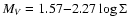 with error estimates (Van Paradijs & McClintock 1994).
An additional error term of 0.5 mag representing inclination
variations is added to the original error estimates.
To estimate the V magnitude,
an intrinsic color
with error estimates (Van Paradijs & McClintock 1994).
An additional error term of 0.5 mag representing inclination
variations is added to the original error estimates.
To estimate the V magnitude,
an intrinsic color
 is assumed.
The column density of X-ray measurements has been used to estimate
the extinction
AV = 1.8
and color excess
EB-V = AV/3 = 0.6 The horizontal lines are upper limits for the distance
assuming
is assumed.
The column density of X-ray measurements has been used to estimate
the extinction
AV = 1.8
and color excess
EB-V = AV/3 = 0.6 The horizontal lines are upper limits for the distance
assuming
 (for a 1.5
  NS and a He-rich donor)
and 15 kpc distance from the Galactic Center.
Note that the galactic latitude implies a distance of
NS and a He-rich donor)
and 15 kpc distance from the Galactic Center.
Note that the galactic latitude implies a distance of
 from the Galactic Plane.
Constant-period lines represented by solid (P = 36 min) and
dashed lines (P = 80 min) indicate the region of degenerate
donors. Systems with periods below 36 min and observable accretion
rates are most likely produced by tidal capture.
It seems possible that the system has a very short period.
from the Galactic Plane.
Constant-period lines represented by solid (P = 36 min) and
dashed lines (P = 80 min) indicate the region of degenerate
donors. Systems with periods below 36 min and observable accretion
rates are most likely produced by tidal capture.
It seems possible that the system has a very short period. |
| Open with DEXTER |
The galactic coordinates of 4U 1543-624 (
and
)
imply a minimum distance between the source and Galactic Center of
 (assuming a distance of 8.6 kpc for the
Galactic Center).
Therefore 4U 1543-624 is probably a member of the disk population,
and the common literature value of distance
(assuming a distance of 8.6 kpc for the
Galactic Center).
Therefore 4U 1543-624 is probably a member of the disk population,
and the common literature value of distance
 ,
more representative for the bulge population,
should be regarded as an order-of-magnitude estimate.
Using the empirical relation between optical and X-ray fluxes and
the period (Van Paradijs & McClintock 1994), it can be concluded that the system may
have a degenerate donor (Fig. 3),
and the distance is likely to be in the range
3-
,
more representative for the bulge population,
should be regarded as an order-of-magnitude estimate.
Using the empirical relation between optical and X-ray fluxes and
the period (Van Paradijs & McClintock 1994), it can be concluded that the system may
have a degenerate donor (Fig. 3),
and the distance is likely to be in the range
3-
 .
.
Archival X-ray observations of 4U 1543-624 have been analyzed.
The X-ray continuum can be fitted with a two-component model consisting
of an isothermal blackbody and a Comptonized component.
Two different X-ray states are seen. In the high state, the luminosity
comes mainly from the Comptonized component and the spectrum is
harder. The low state spectrum is dominated by the BB,
but the Comptonized component is also important at
energies below
 .
Two Gaussian features at
(the Fe
line) and
are detected. The Fe
line
is seen only in the high state, and it has at least
one order of magnitude lower flux in the low state.
A two-layer disk, with
the lower and cooler layer providing the input photons
to be upscattered by the hotter surface layer,
provides a qualitative explanation for the X-ray continuum
and state transitions.
.
Two Gaussian features at
(the Fe
line) and
are detected. The Fe
line
is seen only in the high state, and it has at least
one order of magnitude lower flux in the low state.
A two-layer disk, with
the lower and cooler layer providing the input photons
to be upscattered by the hotter surface layer,
provides a qualitative explanation for the X-ray continuum
and state transitions.
The BB component of the X-ray spectrum
can be taken as weak evidence of a neutron star. It is probably
safe to assume that the BB comes from a boundary
layer between the neutron star surface and the inner disk,
and the Comptonized component is from a hot disk corona.
The ratio of the continuum component luminosities is close to unity.
This is in good accordance with the theoretical expectation for
a slowly rotating neutron star (Sunyaev & Shakura 1986). Most LMXBs
have lower BB luminosities (White et al. 1988).
A rapidly rotating neutron star or non-thermal emission from
the boundary layer have been suggested to explain this discrepancy.
In LMXBs with detected BB emission, the
BB luminosity correlates strongly with total luminosity.
The BB luminosity of 4U 1543-624 decreases slightly
when the total luminosity increases significantly.
The changes seen in continuum spectrum and its variations,
which are oppposite to observations of other LMXBs,
can be explained if 4U 1543-624 has
a boundary layer with a spectrum close to BB and
a slowly rotating neutron star (
 ).
).
Angular momentum of the accreted matter tends to spin up the
neutron stars. An equilibrium between angular momentum gain
from the accretion flow and losses due to gravitational radiation
is reached at periods of the order one millisecond.
For typical LMXB accretion rates the equilibrium is reached
in a time of the order 107 years (Rappaport et al. 1983).
The observations suggest that 4U 1543-624 has gained less angular momentum.
It has either been accreting for a shorter time than a typical LMXB,
or the accretion rate is significantly smaller.
Monitoring observations with sufficient energy resolution to estimate
the continuum components would be especially useful.
Such observations have the best possibility of observing
the system in a wide range of states.
The Gaussian feature seen in the RXTE high state spectra
near
is interpreted as the Fe
line.
The line parameters are partially produced by instrumental
effects, and should be treated with some caution.
As the line is absent in the low state,
with an upper flux limit one order of
magnitude lower than the observed RXTE flux, the line
is probably related to the Comptonized component.
The line is broad and the centroid energy is above
the neutral iron value, suggesting it might originate from
ionized gas. Possible mechanisms producing this line are radiative
recombination (Arnaud & Raymond 1992), collisional excitation (Arnaud & Rothenflug 1985)
and Compton reflection (Magdziarz & Zdziarski 1995). The line width implies
fluorescence is less likely to be responsible for the line.
High S/N low-state spectra are needed to provide better constraints
on the line formation. If the low-state Fe
fluxes are close
to the upper limit derived from ASCA data, more detailed modeling
than presented here is needed. On the other hand, very low
line fluxes would favour the Compton reflection mechanism.
The two-layer disk model providing the best qualitative explanation
for the Comptonized spectrum could easily produce such
a reflected component.
The
feature has been detected previously in
ASCA data (Juett et al. 2001). It also detected in SAX data,
and the parameters do not change significantly, when a different
continuum model is used. This analysis confirms the detection of the
feature.
The feature is either a neon absorption
edge, made stronger by enhanced neon abundace (Juett et al. 2001),
or an emission line. Juett et al. (2001) suggest
observations with very high spectral resolution
to distinguish between the two mechanisms producing the feature.
The detected state transitions show that the distinction could also
be made by comparing medium-resolution observations in the
two states. If the feature strength changes with state, the
line interpretation is more likely. Changes in the continuum
component physically related to the line are likely to produce
changes in the line parameters. If the equivalent width of the
feature remains unchanged during state transitions, it is more
likely to be the absorption edge.
Optical spectroscopy of the system would allow determining the
abundances of the inflowing matter. The equivalent
widths of the lines near
 He II, C III, N III
and
H
He II, C III, N III
and
H could provide the needed abundance diagnostics.
A short-period system with a degenerate donor would
have stronger He and possibly CNO lines and weaker
H
line than a system with a main sequence donor.
could provide the needed abundance diagnostics.
A short-period system with a degenerate donor would
have stronger He and possibly CNO lines and weaker
H
line than a system with a main sequence donor.
Acknowledgements
I am grateful to Pasi Hakala, Panu Muhli
and Osmi Vilhu for useful discussions, and to Diana Hannikainen for
both useful discussions and checking the English of the manuscript.
I thank the anonymous referee for his/her useful comments.
This research has made use of NASA's Astrophysics Data System (ADS)
Bibliographic Services and data obtained from the High Energy
Astrophysics Science Archive Research Center (HEASARC), provided
by NASA's Goddard Space Flight Center, and
the SIMBAD database, operated at CDS, Strasbourg, France.
Financial support of Academy of Finland and the National
Technology Agency TEKES is acknowledged.
- Apparao, K. M. V., Bradt, H. V., Dower, R. G., et al.
1978, Nature, 271, 225
In the text
NASA ADS
- Arnaud, K. A. 1996,
in Astronomical Data Analysis Software Systems V, ed. G. Jacoby, J. & Barnes
(San Fransisco: ASP), ASP Conf. Ser., 101, 17
In the text
-
Arnaud, M., & Raymond, J. 1992, ApJ, 392, 394
In the text
-
Arnaud, M., & Rothenflug, R. 1985, A&AS, 60, 425
In the text
NASA ADS
- Asai, K., Dotani, T.,
Nagase, F., & Mitsuda, K. 2000, ApJS, 131, 571
In the text
NASA ADS
-
Boella, G., Chiappetti, L., Conti, G., et al. 1997, A&AS, 122, 327
In the text
NASA ADS
-
Bohlin, R. C., Savage, B. D., & Drake, J. H. 1978, ApJ, 224, 132
In the text
NASA ADS
- Bradt, H. V., Rothschild, R. E., &
Swank, J. H. 1993, A&AS, 97, 355
In the text
NASA ADS
-
Christian, D. J., & Swank, J. H. 1997, ApJS, 109, 177
In the text
NASA ADS
-
Church, M. J., Inogamov, N. A., & Balucinska-Church, M. 2002,
A&A, 390, 139
In the text
NASA ADS
-
Dickey, J. M., & Lockman, F. J. 1990, ARA&A, 28, 215
In the text
NASA ADS
- Emelyanov, A. N.,
Aleksandovich, N. L., & Sunyaev, R. A. 2000, Astro. Lett., 26, 297
In the text
NASA ADS
- Fiore, F., Guainazzi, M. & Grandi, P. 1999,
Cookbook for BeppoSAX NFI Spectral Analysis, available by ftp from
In the text
legacy.gsfc.nasa.gov/sax/doc/software_docs/saxabc_v1.2.ps
- Forman, W., Jones, C.,
Cominsky, L., et al. 1978, ApJS, 38, 357
In the text
NASA ADS
- Frontera, F., Costa, E., dal Fiume,
D., et al. 1997, A&AS, 122, 357
In the text
NASA ADS
- Gottwald, M., Parmar, A. N.,
Reynolds, A. P., et al. 1995, A&AS, 109, 9
In the text
NASA ADS
-
Inogamov, N. A., & Sunyaev, R. A. 1999, Astro. Lett., 25, 269
NASA ADS
-
Jahoda, K., Swank, J. H., Giles, A. B., et al. 1996, Proc. SPIE, 2808, 59
In the text
-
Juett, A. M., Psaltis, D., & Chakrabarty, D. 2001, ApJ, 560, L59
In the text
NASA ADS
- Kallman, T. R. 1995, ApJ, 455, 603
In the text
NASA ADS
-
Levine, A. M., Bradt, H., Cui, W., et al. 1996, ApJ, 469, L33
In the text
NASA ADS
-
Magdziarz, P., & Zdziarski, A. 1995, MNRAS, 273, 837
In the text
NASA ADS
-
Makishima, K., Maejima, Y., Mitsuda, K., et al. 1986, ApJ, 308, 635
In the text
NASA ADS
-
Manzo, G., Giarrusso, S., Santangelo, A., et al. 1997, A&AS, 122, 341
In the text
NASA ADS
- Markert, T. H., Laird, F. N., Clark,
G. W., et al. 1979, ApJS, 39, 573
In the text
NASA ADS
- McClintock, J. E., Canizares, C. R.,
Hiltner, W. A., & Petro, L. 1978, IAUC, 3251
In the text
- Nagase, F. 1989, PASJ, 41, 1
In the text
NASA ADS
- Parmar, A. N., Martin, D. D. E., Bavdaz,
M., et al. 1997, A&AS, 122, 309
In the text
NASA ADS
-
Poutanen, J., & Svensson, R. 1996, ApJ, 470, 249
In the text
NASA ADS
- Predehl, P., & Schmitt, J. H. M. M.
1995, A&A, 293, 889
In the text
NASA ADS
-
Rappaport, S., Verbunt, F., & Joss, P. C. 1983, ApJ, 275, 713
In the text
NASA ADS
- Scargle, J. D. 1982, ApJ, 263, 835
In the text
NASA ADS
- Singh, K. P., Apparao, K. M. V., & Kraft, R. P.
1994, ApJ, 421, 753
In the text
NASA ADS
-
Sunyaev, R. A., & Shakura, N. I. 1986, Sov. Astron. Lett., 12, 117
In the text
NASA ADS
-
Sunyaev, R., & Titarchuk, L. 1980, A&A, 86, 121
In the text
NASA ADS
-
Tanaka, Y., Inoue, H., & Holt, S. S. 1994, PASJ, 46, L37
NASA ADS
-
Tanaka, Y., & Lewin, W. H. G. 1995, in X-ray binaries, ed.
W. H. G. Lewin, J. van Paradijs, & E. P. J. van den Heuvel (Cambridge
University press)
In the text
- Titarchuk, L. 1994, ApJ, 434, 313
In the text
- Van Paradijs, J., &
McClintock, J. E. 1994, A&A, 290, 133
In the text
NASA ADS
- Van Paradijs, J., &
McClintock, J. E. 1995, in X-ray binaries, ed.
W. H. G. Lewin, J. van Paradijs, & E. P. J. van den Heuvel (Cambridge
University press)
In the text
- Warwick, R. S.,
Marshall, N., Fraser, G. W., et al. 1981, MNRAS, 197, 865
In the text
NASA ADS
- White, N. E., Stella, L., & Parmar,
A. N. 1988, ApJ, 324, 363
In the text
NASA ADS
- Wood, K. S., Meekins, J. F., Yentis,
D. J., et al. 1984, ApJS, 56, 507
In the text
NASA ADS
Copyright ESO 2003
![\begin{figure}
\par\includegraphics[angle=270,width=8.8cm,clip]{H3816_F1.eps} \end{figure}](/articles/aa/full/2003/01/aah3816/img22.gif)
![\begin{figure}
\par\includegraphics[angle=270,width=8.8cm,clip]{H3816_F2.eps} \end{figure}](/articles/aa/full/2003/01/aah3816/img101.gif)
![\begin{figure}
\par\includegraphics[width=8.8cm,clip]{H3816_F3.eps}\end{figure}](/articles/aa/full/2003/01/aah3816/img117.gif)