Wave propagation in a zero-
A&A 396, 993-1002 (2002)
DOI: 10.1051/0004-6361:20021296
K. Karami 1 - S. Nasiri1,2 - Y. Sobouti1,3
1 - Institute for Advanced Studies in Basic Sciences, Gava Zang, Zanjan 45195, Iran
2 -
Department of Physics, Zanjan University, Zanjan, Iran
3 -
Center for Theoretical Physics and Mathematics,
AEOI, PO Box 11345-8486, Tehran, Iran
Received 19 April 2002 / Accepted 25 June 2002
Abstract
Wave propagation in a zero-![]() magnetic flux tube with a
discontinuous Alfvèn speed at its surface is considered. The
problem is reduced to solving a wave equation for the projection
of the magnetic perturbation along the axis of the cylinder. The
mathematical formalism is identical with that for the propagation
of electromagnetic waves in optical fibers with a varying index of
refraction in the cross section of the fiber. The dispersion
relation is solved in its full generality and three wave numbers
are assigned to the normal modes of the cylinder. There is a lower
cutoff for the longitudinal wave number along the cylinder axis
and an upper cutoff for the radial wave number. Eigenfrequencies
and eigenfields (i.e. the magnetic and velocity fields of modes)
are calculated. Resistive and viscous dissipation rates have
mathematically identical forms, differing only in their being
inversely proportional to the Lundquist and Reynolds numbers,
respectively. These rates as well as the energy densities are
obtained for each mode and are commented on.
magnetic flux tube with a
discontinuous Alfvèn speed at its surface is considered. The
problem is reduced to solving a wave equation for the projection
of the magnetic perturbation along the axis of the cylinder. The
mathematical formalism is identical with that for the propagation
of electromagnetic waves in optical fibers with a varying index of
refraction in the cross section of the fiber. The dispersion
relation is solved in its full generality and three wave numbers
are assigned to the normal modes of the cylinder. There is a lower
cutoff for the longitudinal wave number along the cylinder axis
and an upper cutoff for the radial wave number. Eigenfrequencies
and eigenfields (i.e. the magnetic and velocity fields of modes)
are calculated. Resistive and viscous dissipation rates have
mathematically identical forms, differing only in their being
inversely proportional to the Lundquist and Reynolds numbers,
respectively. These rates as well as the energy densities are
obtained for each mode and are commented on.
Key words: Sun: corona - magnetohydrodynamics (MHD) - Sun: magnetic fields - Sun: oscillations
Since the discovery of the hot solar corona about sixty years ago,
different theories of coronal heating have been put forward and
debated. Recent observations, however, have indicated the
existence of magnetohydrodynamic (mhd) waves and their damping in
coronal loops and suggest they may be sources of heat supply to
the corona. In their analysis of observations by the Transition
Region and Coronal Explorer (TRACE), Nakariakov et al. (1999)
reported the detection of spatial oscillations in five coronal
loops with periods ranging from 258 to 320 s. They interpreted
them as global mhd standing waves driven by solar flares in the
adjacent active regions. TRACE also detected decaying oscillations
in a long,
![]() m, and thin,
m, and thin,
![]() m, bright coronal loop in the 171 Å emission lines of FeIX. The decay time was
m, bright coronal loop in the 171 Å emission lines of FeIX. The decay time was
![]() min for an oscillation of
min for an oscillation of
![]() millihertz. All these observations indicate strong dissipation of
the wave energy that may be the cause of coronal heating.
millihertz. All these observations indicate strong dissipation of
the wave energy that may be the cause of coronal heating.
Resonant absorption of Alfvèn waves in coronal inhomogeneities
was first suggested by Ionson (1978) as a nonthermal mechanism of
heating. He pointed out the importance of the density and magnetic
field gradients in dissipating the wave energy. Ionson's
conclusions received further support from the more extensive
calculations of Hollweg (1984). Wentzel (1979a,b) was among the
early investigators studying the propagation and dissipation of
mhd waves along surfaces of discontinuity of Alfvèn speeds.
Wilson (1979, 1980) studied the vibrational modes of flux sheaths
and flux tubes embedded in compressible but unstratified
atmospheres and obtained a general dispersion relation. Roberts
(1981a,b) proposed the occurrence of magnetoacoustic surface
waves along magnetic interfaces. Edwin ![]() Roberts (1983)
elaborated on the dispersion relation for a magnetic cylinder
embedded in a magnetic environment typical of that of the solar
photosphere and corona. Roberts et al. (1984) found two
distinct time scales (long acoustic and short Alfvèn ones) for
the propagation of magnetoacoustic waves in coronal
inhomogeneities. Steinolfson et al. (1986) were concerned with the
role of viscous and resistive dissipations on surface waves in
cases of both continuous and discontinuous variations of
Alfvèn speeds. Davila (1987) and Steinolfson
Roberts (1983)
elaborated on the dispersion relation for a magnetic cylinder
embedded in a magnetic environment typical of that of the solar
photosphere and corona. Roberts et al. (1984) found two
distinct time scales (long acoustic and short Alfvèn ones) for
the propagation of magnetoacoustic waves in coronal
inhomogeneities. Steinolfson et al. (1986) were concerned with the
role of viscous and resistive dissipations on surface waves in
cases of both continuous and discontinuous variations of
Alfvèn speeds. Davila (1987) and Steinolfson ![]() Davila
(1993) did much analytic and numerical work on resonant absorption
and of their resistive dissipation. Ofman et al. (1994, 1995)
included viscous dissipation in their analysis and concluded that
the shear viscous dissipation is of the same magnitude as the
resistive heating. Contribution of the compressional viscosity,
however, was found to be insignificant.
Davila
(1993) did much analytic and numerical work on resonant absorption
and of their resistive dissipation. Ofman et al. (1994, 1995)
included viscous dissipation in their analysis and concluded that
the shear viscous dissipation is of the same magnitude as the
resistive heating. Contribution of the compressional viscosity,
however, was found to be insignificant.
Here we study a cylindrical magnetic flux tube with a
discontinuous Alfvèn speed across the surface of cylinder. The
model is essentially the same as that of Edwin ![]() Roberts (1983)
but without limiting it to slender tubes. In Sect. 2 we reduce the
problem to solving a wave equation for the component of the
magnetic field along the cylinder axis and discuss the relevant
boundary conditions. In Sect. 3 we elaborate on the dispersion
relation, give its graphical and numerical solutions, and
introduce cutoffs. In Sect. 4 we discuss resistive and viscous
dissipations. In Sects. 5 and 6 we give further numerical and
graphical results. Section 7 is devoted to concluding remarks.
Lengthy formulae are collected in Appendix A. Purely transverse
modes, with no longitudinal components in magnetic and velocity
fields, have certain peculiarities. They are touched upon in
Appendix B.
Roberts (1983)
but without limiting it to slender tubes. In Sect. 2 we reduce the
problem to solving a wave equation for the component of the
magnetic field along the cylinder axis and discuss the relevant
boundary conditions. In Sect. 3 we elaborate on the dispersion
relation, give its graphical and numerical solutions, and
introduce cutoffs. In Sect. 4 we discuss resistive and viscous
dissipations. In Sects. 5 and 6 we give further numerical and
graphical results. Section 7 is devoted to concluding remarks.
Lengthy formulae are collected in Appendix A. Purely transverse
modes, with no longitudinal components in magnetic and velocity
fields, have certain peculiarities. They are touched upon in
Appendix B.
More often than not, magnetohydrodynamic (mhd) waves propagating
in coronal loops have, mathematically, the same structure as the
light signals propagating in optical fibers and/or dielectric
resonators, a point addressed by Nakariakov ![]() Roberts (1995) and Nakariakov (2000). For example, in
a cylindrical fiber lying in the z-direction with a graded or
step-like index of refraction, the electromagnetic fields
Roberts (1995) and Nakariakov (2000). For example, in
a cylindrical fiber lying in the z-direction with a graded or
step-like index of refraction, the electromagnetic fields
![]() and
and ![]() can be expressed in terms of Ezor Bz depending on whether the mode in question is a
transverse magnetic or a transverse electric one. Similarly, in a
low-
can be expressed in terms of Ezor Bz depending on whether the mode in question is a
transverse magnetic or a transverse electric one. Similarly, in a
low-![]() magnetic flux tube with graded or step-like Alfvèn
speed, propagation of fast magnetoacoustic waves can be reduced to
solving a wave equation for the z-component of the perturbation
in the magnetic field. In both cases the differential equations
for z-components of fields are identical. The boundary
conditions, however, differ. See e.g. Ghatak
magnetic flux tube with graded or step-like Alfvèn
speed, propagation of fast magnetoacoustic waves can be reduced to
solving a wave equation for the z-component of the perturbation
in the magnetic field. In both cases the differential equations
for z-components of fields are identical. The boundary
conditions, however, differ. See e.g. Ghatak ![]() Thyagarajan
(1998) for light propagation in optical fibers.
Thyagarajan
(1998) for light propagation in optical fibers.
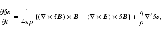
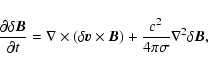
The linearized mhd equations for a zero-![]() plasma are
plasma are
 |
(1) |
 |
(2) |
We let the flux tube lie along the z-axis and let
![]() and
and
![]() ,
where
,
where
![]() is the coordinate vector transverse to the
magnetic field. That
is the coordinate vector transverse to the
magnetic field. That ![]() is independent of z follows from the
assumption of an unstratified tube. That
is independent of z follows from the
assumption of an unstratified tube. That ![]() is a
consequence of
is a
consequence of
![]() .
We further assume
an exponential z- and t-dependence, e
.
We further assume
an exponential z- and t-dependence, e
![]() ,
for any of the components
,
for any of the components
![]() and
and
![]() .
We take the following steps: i) Take the
time derivative of Eq. (2) and substitute for
.
We take the following steps: i) Take the
time derivative of Eq. (2) and substitute for
![]() from Eq. (1). ii) Decompose the resulting
equation into its z- and transverse components. We arrive at
from Eq. (1). ii) Decompose the resulting
equation into its z- and transverse components. We arrive at
| (3) |
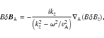 |
(4) |
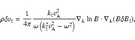 |
(5) |
 |
(6) |
Equations (3)-(6) become singular if
![]() at some point r. The singularity can, however, be removed by the
introduction of any dissipation mechanism. This issue is addressed
in ample detail by Ionson (1978), Davila (1987), Steinolfson &
Davila (1993), Ofman et al. (1994, 1995), Kivelson & Russell
(1997), Roberts & Ulmschneider (1997), and Nakariakov (2000).
at some point r. The singularity can, however, be removed by the
introduction of any dissipation mechanism. This issue is addressed
in ample detail by Ionson (1978), Davila (1987), Steinolfson &
Davila (1993), Ofman et al. (1994, 1995), Kivelson & Russell
(1997), Roberts & Ulmschneider (1997), and Nakariakov (2000).
Hereafter, we consider a circular cylinder and use cylindrical
coordinates
![]() .
For simplicity, the radius of the
cylinder is taken as the unit of length. The length
of the cylinder is assumed to be
.
For simplicity, the radius of the
cylinder is taken as the unit of length. The length
of the cylinder is assumed to be ![]() in the same unit. To
ensure periodicity in z direction one must then have
kz=l/L,
in the same unit. To
ensure periodicity in z direction one must then have
kz=l/L,
![]() We further assume a constant
magnetic field throughout the space and a step-like mass density,
We further assume a constant
magnetic field throughout the space and a step-like mass density,
![]() for r<1 and
for r<1 and
![]() for r>1. The
condition
for r>1. The
condition
![]() implies
implies
![]() and it
is necessary to have standing waves in the flux tube. Otherwise
any perturbation in the fields will propagate away to infinity.
With these simplifications, Eq. (3) reduces to
and it
is necessary to have standing waves in the flux tube. Otherwise
any perturbation in the fields will propagate away to infinity.
With these simplifications, Eq. (3) reduces to
 |
(7) |
 |
(8) |
 |
(9) |
i) To avoid shock waves at r=1, the Lagrangian changes in
pressure should be continuous. Here, on account of the
zero-![]() approximation and constancy of B throughout space
this reduces to the continuity of
approximation and constancy of B throughout space
this reduces to the continuity of
![]() .
Thus
.
Thus
| (10) |
 |
|||
| (11) |
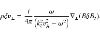
![\begin{figure}
\par\includegraphics[width=10cm,clip]{2597f1.eps} \end{figure}](/articles/aa/full/2002/48/aa2597/img71.gif) |
Figure 1:
The plots of the two sides of Eq. (14), the dispersion relation, as functions of x for
m=0 (sausage modes), m=1 (kink modes), and m=2 (fluting modes) with l=100,
C1002=8.9, radius =103 km,
length =105 km,
and
|
| Open with DEXTER | |
 |
(12) |
| (13) |
 |
(14) |
In thin flux tubes, ![]() ,
approximating Jm(x) and
,
approximating Jm(x) and
![]() as (x/2)m and
(y/2)-m,
as (x/2)m and
(y/2)-m, ![]() ,
gives x=y.
This in turn leads to an approximate dispersion relation
,
gives x=y.
This in turn leads to an approximate dispersion relation
![]() where the average Alfvèn speed,
the same as the kink speed of Edwin
where the average Alfvèn speed,
the same as the kink speed of Edwin ![]() Roberts (1983), is
obtained from
Roberts (1983), is
obtained from
![]() .
For m=0,
however, this approach breaks down, because of the logarithmic
behavior of K0(y) at small y. Thin flux tubes are studied
in detail by Ionson (1978), Wentzel (1979a,b), Wilson (1979,
1980), Edwin & Roberts (1983), Roberts et al. (1984), Hasan
.
For m=0,
however, this approach breaks down, because of the logarithmic
behavior of K0(y) at small y. Thin flux tubes are studied
in detail by Ionson (1978), Wentzel (1979a,b), Wilson (1979,
1980), Edwin & Roberts (1983), Roberts et al. (1984), Hasan ![]() Sobouti (1987), Nasiri (1992), and Nakariakov et al. (1999).
Sobouti (1987), Nasiri (1992), and Nakariakov et al. (1999).
Asymptotic behavior of xnml: let
![]() and
and
![]() be the nth root of Jm(x) and J'm(x),
respectively. Asymptotically for higher roots one has
be the nth root of Jm(x) and J'm(x),
respectively. Asymptotically for higher roots one has
![]() and
and
![]() .
From Fig. 1 for
.
From Fig. 1 for ![]() ,
it
is clear that
,
it
is clear that
![]() .
Using the
asymptotic form of
.
Using the
asymptotic form of ![]() s one finds
s one finds
 |
(15) |
| = | |||
| (16) |
| = | |||
| = | (17) |
A mode given by Eqs. (16), (17) and (A.1)-(A.4) is characterized by a
trio of wave numbers (n,m,l) that actually count the number of
nodes or antinodes along ![]() ,
and z directions,
respectively. This trio provides a suitable basis for the
classification of modes. What in the literature are termed as
sausage, kink and fluting modes, in the present analysis
correspond to modes with m=0,1 and 2 or greater, respectively.
,
and z directions,
respectively. This trio provides a suitable basis for the
classification of modes. What in the literature are termed as
sausage, kink and fluting modes, in the present analysis
correspond to modes with m=0,1 and 2 or greater, respectively.
| (18) |
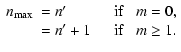
For a given
![]() there exists an upper cutoff,
there exists an upper cutoff, ![]() ,
for the radial wave number. This can be obtained by examining
,
for the radial wave number. This can be obtained by examining
![]() s and finding out which one is closest but smaller
than
s and finding out which one is closest but smaller
than ![]() ;
see again Fig. 1. Then
;
see again Fig. 1. Then
 |
(19) |
![\begin{displaymath}n_{\max}\approx
{\rm integer}(x_{\max}/\pi)={\rm integer}[(\rho_{\rm i}/\rho_{\rm e}-1)^{1/2}l/\pi L],
\end{displaymath}](/articles/aa/full/2002/48/aa2597/img119.gif) |
(20) |
The finite conductivity and viscosity of plasma causes an
exponential time decay of disturbances. For weak dissipations one
may assume
| (21) |
| (22) |
![\begin{displaymath}\alpha_{nml}=\left(\omega_{\rm A}/4\pi\right)\left(S^{-1}+R^{-1}\right)\left[x_{nml}^2+(
l/L)^2\right],~~~~~~r<1,
\end{displaymath}](/articles/aa/full/2002/48/aa2597/img126.gif) |
(23) |
The current density generated by
![]() is
is
![]() .
For a
damped field of Eq. (21), this gives an ohmic heating rate of
.
For a
damped field of Eq. (21), this gives an ohmic heating rate of
![]() .
Similarly the
viscous heating rate is
.
Similarly the
viscous heating rate is
![]() .
For a mode (nml) the integrands are given in Appendix A,
Eq. (A.5). Both turn out to have identical mathematical form,
leaving the ohmic and the viscous contribution to be proportional
to S-1 and R-1, respectively. Correspondingly, the total
dissipation time scale becomes
.
For a mode (nml) the integrands are given in Appendix A,
Eq. (A.5). Both turn out to have identical mathematical form,
leaving the ohmic and the viscous contribution to be proportional
to S-1 and R-1, respectively. Correspondingly, the total
dissipation time scale becomes
![]() .
.
The total heat ![]() ,
generated mainly over one or two total
dissipative time scales, is obtained by a further time integration
of
,
generated mainly over one or two total
dissipative time scales, is obtained by a further time integration
of
![]() .
This, not
surprisingly, turns out to be equal to the total energy initially
vested in the wave in the form of kinetic and magnetic energies.
Thus,
.
This, not
surprisingly, turns out to be equal to the total energy initially
vested in the wave in the form of kinetic and magnetic energies.
Thus,
| = |  |
||
| = |  |
||
| = |  |
||
 |
|||
| + | ![$\displaystyle \left[(l/L)^2-m^2
-\left(\frac{1}{x_{nml}^2}-\frac{1}{y_{nml}^2}\right)(ml/L)^2\right]J_{m}^2(x_{nml})\Bigg\}\cdot$](/articles/aa/full/2002/48/aa2597/img141.gif) |
(24) |
As typical parameters for a coronal loop, we assume radius =
103 km,
![]() km,
km,
![]() ,
,
![]() gr cm-3,
B=100 G,
gr cm-3,
B=100 G,
![]() s-1, and
s-1, and
![]() .
For such a loop one finds
.
For such a loop one finds
![]() km s-1,
km s-1,
![]() km s-1,
km s-1,
![]() rad s-1,
rad s-1,
![]() ,
,
![]() .
The roots xnml and ynml are calculated
and displayed in Tables 1, 2 and 3 for m=0,1, and 2,
respectively. In each table three radial mode numbers n=1,2 and
3, and several longitudinal wave numbers, l, are considered.
Note the positions of cutoffs in Tables 1-3. For example, in Table 1, for n=1,2,3, one finds
.
The roots xnml and ynml are calculated
and displayed in Tables 1, 2 and 3 for m=0,1, and 2,
respectively. In each table three radial mode numbers n=1,2 and
3, and several longitudinal wave numbers, l, are considered.
Note the positions of cutoffs in Tables 1-3. For example, in Table 1, for n=1,2,3, one finds
![]() ,
respectively.
Conversely for
l=58,91,100 one finds
,
respectively.
Conversely for
l=58,91,100 one finds
![]() ,
respectively in compliance with Eqs. (18) and (19). In fact if one
considers the tables as the wave number plane (l,n) the dashed
portion of the plane is the forbidden zone for a normal mode to
exist. Analogs of these features exist for the propagation of
electromagnetic waves in optical fibers.
,
respectively in compliance with Eqs. (18) and (19). In fact if one
considers the tables as the wave number plane (l,n) the dashed
portion of the plane is the forbidden zone for a normal mode to
exist. Analogs of these features exist for the propagation of
electromagnetic waves in optical fibers.
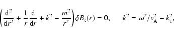
![\begin{figure}
\par\includegraphics[width=11cm,clip]{2597f2.eps} \end{figure}](/articles/aa/full/2002/48/aa2597/img150.gif) |
Figure 2:
Magnetic and velocity field components for m=0 (sausage) modes.
|
| Open with DEXTER | |
| l | xnml | ynml | |||||||
| 25 | - | - | - | - | - | - | |||
| 26 | 2.4191 | - | - | 0.1282 | - | - | |||
| 58 | 2.7718 | - | - | 1.4919 | - | - | |||
| 59 | 2.7793 | 5.5314 | - | 1.5250 | 0.1962 | - | |||
| 91 | 2.9757 | 5.7883 | - | 2.5465 | 2.0049 | - | |||
| 92 | 2.9807 | 5.7937 | 8.6588 | 2.5777 | 2.0436 | 0.1883 | |||
| 100 | 3.0190 | 5.8349 | 8.7444 | 2.8264 | 2.3442 | 1.1196 | |||
| n=1 | n=2 | n=3 | n=1 | n=2 | n=3 |
| l | xnml | ynml | |||||||
| 1 | 0.0284 | - | - | 0.0284 | - | - | |||
| 40 | 0.7865 | - | - | 1.1671 | - | - | |||
| 41 | 0.7984 | 3.8369 | - | 1.1968 | 0.1545 | - | |||
| 74 | 1.0827 | 4.1281 | - | 2.1809 | 1.7803 | - | |||
| 75 | 1.0890 | 4.1347 | 7.0237 | 2.2108 | 1.8157 | 0.2701 | |||
| 100 | 1.2183 | 4.2783 | 7.2106 | 2.9583 | 2.6589 | 1.9237 | |||
| n=1 | n=2 | n=3 | n=1 | n=2 | n=3 |
| l | xnml | ynml | ||||||||
| 1 | 0.0284 | - | - | 0.0284 | - | - | ||||
| 54 | 1.2383 | - | - | 1.5627 | - | - | ||||
| 55 | 1.2541 | 5.1400 | - | 1.5922 | 0.2243 | - | ||||
| 89 | 1.6768 | 5.3727 | - | 2.6016 | 2.0404 | - | ||||
| 90 | 1.6865 | 5.3785 | 8.4230 | 2.6315 | 2.0775 | 0.3380 | ||||
| 100 | 1.7769 | 5.4337 | 8.4934 | 2.9299 | 2.4378 | 1.2985 | ||||
| n=1 | n=2 | n=3 | n=1 | n=2 | n=3 |
| l |
|
|
|||||||
| 25 | - | - | - | - | - | - | |||
| 26 | 2.5533 | - | - | 0.5188 | - | - | |||
| 58 | 3.3171 | - | - | 0.8756 | - | - | |||
| 59 | 3.3407 | 5.8337 | - | 0.8881 | 2.7081 | - | |||
| 91 | 4.1264 | 6.4558 | - | 1.3550 | 3.3166 | - | |||
| 92 | 4.1518 | 6.4746 | 9.1285 | 1.3717 | 3.3359 | 6.6311 | |||
| 100 | 4.3571 | 6.6267 | 9.2916 | 1.5107 | 3.4947 | 6.8703 | |||
| n=1 | n=2 | n=3 | n=1 | n=2 | n=3 |
| l |
|
|
|||||||
| 1 | 0.0434 | - | - | 0.0001 | - | - | |||
| 40 | 1.4829 | - | - | 0.1750 | - | - | |||
| 41 | 1.5154 | 4.0473 | - | 0.1827 | 1.3035 | - | |||
| 74 | 2.5646 | 4.7377 | - | 0.5234 | 1.7862 | - | |||
| 75 | 2.5957 | 4.7589 | 7.4084 | 0.5361 | 1.8022 | 4.3675 | |||
| 100 | 3.3695 | 5.3079 | 7.8652 | 0.9035 | 2.2420 | 4.9228 | |||
| n=1 | n=2 | n=3 | n=1 | n=2 | n=3 |
| l |
|
|
|||||||
| 1 | 0.0434 | - | - | 0.0001 | - | - | |||
| 54 | 2.1003 | - | - | 0.3510 | - | - | |||
| 55 | 2.1350 | 5.4226 | - | 0.3627 | 2.3399 | - | |||
| 89 | 3.2602 | 6.0567 | - | 0.8458 | 2.9192 | - | |||
| 90 | 3.2922 | 6.0764 | 8.8849 | 0.8625 | 2.9382 | 6.2820 | |||
| 100 | 3.6093 | 6.2766 | 9.0558 | 1.0366 | 3.1350 | 6.5260 | |||
| n=1 | n=2 | n=3 | n=1 | n=2 | n=3 |
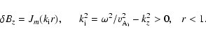
![\begin{figure}
\par\includegraphics[width=11cm,clip]{2597f3.eps} \end{figure}](/articles/aa/full/2002/48/aa2597/img153.gif) |
Figure 3:
Magnetic and velocity field components for m=1 (kink) modes.
|
| Open with DEXTER | |
To acquaint oneself with the characteristics of the magnetic and
velocity fields of the modes we give some sample plots. By Eqs. (A3-4)
![]() ,
and
,
and
![]() and
and
![]() are proportional and opposite to
are proportional and opposite to
![]() and
and
![]() ,
respectively. All components of
,
respectively. All components of
![]() and
and
![]() are plotted in Figs. 2 to 4. In accordance
with the boundary conditions of Eqs. (10), (11), the r- and
z-components are continuous at r=1 but have discontinuous
slopes. The
are plotted in Figs. 2 to 4. In accordance
with the boundary conditions of Eqs. (10), (11), the r- and
z-components are continuous at r=1 but have discontinuous
slopes. The ![]() -component and its slope are both discontinuous.
The amplitudes are highly evanescent outside the tube and maybe
neglected for all practical purposes, for instance, in considering
the heating of corona. The number of nodes in each case is n.
The antinodes of
-component and its slope are both discontinuous.
The amplitudes are highly evanescent outside the tube and maybe
neglected for all practical purposes, for instance, in considering
the heating of corona. The number of nodes in each case is n.
The antinodes of
![]() coincide with the nodes of
coincide with the nodes of
![]() ;
for,
;
for,
![]() is proportional to the derivative of
is proportional to the derivative of
![]() ;
see Eq. (A.1). The converse is, however, not true.
The nodes of
;
see Eq. (A.1). The converse is, however, not true.
The nodes of
![]() and
and
![]() occur at the
same place, for they are proportional to each other. See Eqs. (17)
and (A.2). For m=1, however, there is an exception. At r=0,
occur at the
same place, for they are proportional to each other. See Eqs. (17)
and (A.2). For m=1, however, there is an exception. At r=0,
![]() is finite and
is finite and
![]() has a node.
has a node.
The velocity field has no z-component. Its transverse
components,
![]() ,
are proportional and
opposite in direction to
,
are proportional and
opposite in direction to
![]() ,
and have the
same graphical representations. It should be remarked, however,
that, because of i in Eqs. (4), (6), (A.1) and (A.3) the phase
of
,
and have the
same graphical representations. It should be remarked, however,
that, because of i in Eqs. (4), (6), (A.1) and (A.3) the phase
of
![]() and
and
![]() differ from those of
differ from those of
![]() ,
,
![]() ,
and
,
and
![]() by
by ![]() .
.
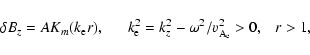
The densities of viscous and ohmic dissipation, Eq. (A.5) and the
integrand in Eq. (24) are plotted in Fig. 5. Comparing Fig. 5 with
Figs. 2 to 4, one concludes that the highest and the lowest
heating rates occur at the antinodes and nodes of
![]() and
and
![]() ,
respectively. In regions exterior to the flux
tube, r>1, the energy densities sharply drop to zero, supporting
the assertion that the wave energy and heat dissipations are not
of significance in the outer regions.
,
respectively. In regions exterior to the flux
tube, r>1, the energy densities sharply drop to zero, supporting
the assertion that the wave energy and heat dissipations are not
of significance in the outer regions.
![\begin{figure}
\par\includegraphics[width=11cm,clip]{2597f4.eps} \end{figure}](/articles/aa/full/2002/48/aa2597/img157.gif) |
Figure 4: Magnetic and velocity field components for m=2 (fluting) modes. Legend and auxiliary parameters as in Fig. 3. |
| Open with DEXTER | |
![\begin{figure}
\par\includegraphics[width=11cm,clip]{2597f5.eps} \end{figure}](/articles/aa/full/2002/48/aa2597/img159.gif) |
Figure 5:
Densities of ohmic and viscous dissipations
|
| Open with DEXTER | |
For weak viscous and ohmic dissipations, time-decay exponents are
calculated for each mode. The density of heat production rates as
functions of r are the same for both mechanisms. Their
contributions, however, are inversely proportional to the Reynolds
and Lundquist numbers, R and S, respectively. The total
dissipation time scale becomes proportional to
(R-1+S-1).
The total generated heat is, of course, equal to the total initial
energy of the wave. We cannot asses the actual values of
resistivity and viscosity prevailing in coronal regions. One,
however, finds the following
values quoted in the literature:
Steinolfson & Davila (1993) use the values S=103, 104, and 105. Ofman et al. (1994) assume S=104 and R=560 in active
coronal regions and S=104 and R=0.56, otherwise. Viscosity in
their analysis is compressional.
Nakariakov et al. (1999) predict S=1013 and R=1014 on
theoretical grounds and report
S=105-5.8 and
R=105.3-6.1from observational evidence.
The values
![]() employed in the present paper is
for an academic exercise and no further significance should be
attached to it.
employed in the present paper is
for an academic exercise and no further significance should be
attached to it.
Acknowledgements
This work was supported by the Institute for Advanced Studies in Basic Sciences, Zanjan. The authors wish to thank Prof. Wentzel, Prof. Ofman and Dr. Nakariakov for providing valuable consultations.
| = | |||
| = | (A.1) |
| = | |||
| = | (A.2) |
| (A.3) |
| (A.4) |
| |
|||
| |
(A.5) |
| |
= | ||
| = | |||
| = | (A.6) |
 |
(A.7) |
 |
(A.8) |
 |
+ |  |
|
| x=xnml, | (A.9) |
 |
- |  |
|
| y=ynml. | (A.10) |
Setting
![]() in Eqs. (1)-(2) in the absence of
dissipation leads to
in Eqs. (1)-(2) in the absence of
dissipation leads to
 |
(B.1) |
 |
(B.2) |
![\begin{displaymath}{\vec n}\cdot\left[\delta{\vec B}_{\rm i}(c){\rm e}^{-i\omega...
...\delta{\vec B}_{\rm e}(c){\rm e}^{-i\omega_{\rm e}t}\right]=0,
\end{displaymath}](/articles/aa/full/2002/48/aa2597/img191.gif) |
(B.3) |
| (B.4) |