6 Results: Multispectral views of the LMC

This paper mainly deals with the techniques that went into the construction of the MC2. It shows how essential a tool the cross-matching of large surveys is, to derive results on their internal accuracy. The broad range of magnitudes covered by the MC2, as well as the large number of sources involved, allow a multi-wavelength and statistical study of the stellar populations of the Clouds. We present a few results concerning their location in several colour-magnitude and colour-colour diagrams, in order to demonstrate the usefulness of such an optical/infrared catalogue and its relevance in the framework of the Virtual Observatory. Note that observations of cross-matched sources were not simultaneously performed so those following diagrams should be considered as indicative because the colours might not represent correctly variable sources.

6.1 The (K$_{\sf s}$, J-K$_{\sf s}$) colour-magnitude diagram

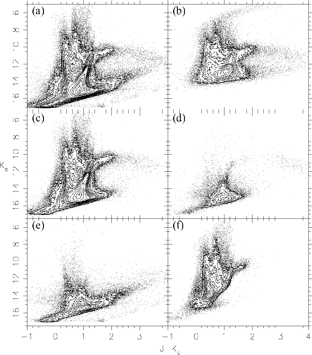
Figure 11a shows the ($K_{\rm s}$, J-$K_{\rm s}$) diagram for all the 2MASS point sources. The total number of sources, nearly two millions, was so large that we chose to plot them as isodensity curves, so as to emphasize different loci of stars. The same technique has been adopted for most of the following diagrams. Unfortunately, this process tends to hide regions with low density of stars. Sources in regions with density lower than the value of the lowest contour level have been plotted as single dots.

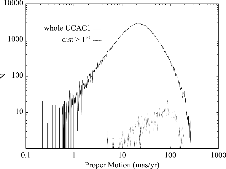
Figure 9: Results of the cross-matching between the UCAC1 and the MC2 catalogues. Histogram of distances to the nearest neighbour. The bin size is 0.1 $^{\prime \prime }$.

The 2MASS colour-magnitude diagram (CMD) has been described in details by Nikolaev & Weinberg (2000), and it will be taken as a reference for the further discussion on the stellar populations obtained from the MC2. Figure 11b is a similar CMD, but for all the DCMC point sources. Figure 11c shows the CMD of the point sources that do have a counterpart in all three catalogues: DCMC, 2MASS and GSC2.2. Figure 11d shows the CMD of all the point sources detected in both DCMC and 2MASS, but not GSC2.2. For Figs. 11c and d the J and $K_{\rm s}$ magnitudes are from 2MASS, including DCMC sources detected only in I and J.

All the 2MASS sources that do not have any counterpart have been plotted on the CMD of Fig. 11e. This feature is a mix of Asymptotic Giant Branch (AGB) and Red Giant Branch (RGB) stars. The position of the AGB bump, located at the bottom of the AGB phase (see Gallart 1998 and references therein), was found by Nikolaev & Weinberg (2000) in the deep 2MASS observations at $K_{\rm s}=15.8$ and (J- $K_{\rm s})=0.7$. The AGB bump stellar population has been well identified by Alcock et al. (2000) thanks to their 9 million LMC stars resulting from the MACHO project. Note that Beaulieu & Sackett (1998) call them the Supraclump. The sensitivity limit is too low here to detect it, as for the red clump, which is located more than one magnitude below the AGB bump ( $K_{\rm s}\sim17$ and (J- $K_{\rm s}) \sim 0.65$, Nikolaev & Weinberg 2000).

Figure 11f refers to sources detected in both 2MASS and UCAC1. It shows mainly a concentration of stars around (J- $K_{\rm s})=0.5$ and $K_{\rm s}=14$, which falls into region D of Nikolaev & Weinberg (2000). Note that Nikolaev & Weinberg (2000) associate the blue half part of region D with G-M dwarfs of the Galaxy. Ruphy et al. (1997) investigated the separation in (J-$K_{\rm s}$) between dwarfs and giants, with the help of early DENIS data, in the direction of the anticenter. They find that roughly for (J- $K_{\rm s})\leq0.6$ there could not be any giants. However, K and M dwarfs may be present for redder colours, together with the giants. RGB stars at the tip of the RGB and AGB stars both O-rich and C-rich can be distinguished at (J- $K_{\rm s})\geq1.0$ (Cioni et al. 2000c).

Figure 10: Results of the cross-matching between the UCAC1 and the MC2 catalogues. Histogram of the proper motions. Both axes have logarithmic scale and the bin size is also logarithmic. The dashed line refers to the cross-matched sources with distances larger than $1^{\prime \prime }$. Their distribution is in the region of sources with large proper motions, when compared to the whole UCAC1 distribution (solid line).

Figure 11: a) ($K_{\rm s}$, J-$K_{\rm s}$) 2MASS CMD: 1 996 448 entries. b) ($K_{\rm s}$, J-$K_{\rm s}$) DENIS CMD: 298 928 entries. c) Point sources present in 2MASS, DCMC and GSC2.2: 1 161 701 entries. The J and $K_{\rm s}$ bands are from 2MASS. d) Point sources detected in 2MASS, DCMC but not GSC2.2: 54 579 entries. The J and $K_{\rm s}$ bands are from 2MASS. e) Point sources detected in 2MASS only: 151 120 entries. f) Point sources detected in both the IR catalogues and UCAC1: 192 848 entries. The J and $K_{\rm s}$ bands are from 2MASS.

6.2 The (J-H, H-K$_{\sf s}$) colour-colour diagram

The (J-H, H-$K_{\rm s}$) diagram may be used to discriminate between dwarf and giant stars, at least to find the bifurcation between M dwarfs and M giants (Bessel & Brett 1988). Dwarfs are on the bluest peak, whereas giants are on the reddest one. This diagram contains only point sources with photometric errors on J, H and $K_{\rm s}$ smaller than 0.06 mag. The (J-H, H-$K_{\rm s}$) diagram is also suitable to isolate reddened stars. Nikolaev & Weinberg (2000) provide such a diagram and label the areas of unusual objects such as Wolf-Rayet stars, protostars, AGB C-rich stars and Be stars. Frogel et al. (1990) surveyed several Magellanic Cloud clusters and overplotted on their resulting (J-H, H-$K_{\rm s}$) diagram the mean relations for globular cluster and field giants. The distribution of their cluster M giants is spread between these two lines, which they relate to a metallicity effect. This could provide an explanation to the slight shift between the giant peak in Fig. 12 and the giant track from Wainscoat et al. (1992) overplotted on it. Finlator et al. (2000) cross-matched 2MASS with SDSS, thus selecting stars on their optical colours and then tracing them in infrared diagrams. They found out that the dwarf peak in the (J-H, H-$K_{\rm s}$) diagram is associated with stars earlier than G5, whereas the giant peak is associated with stars later than K5. This is a typical example illustrating the usefulness of the combination of optical with infrared colours, in order to separate stars according to their spectral type.

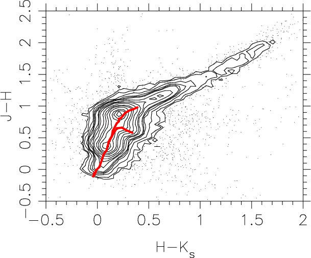Figure 12: Point sources detected in 2MASS, whatever the detection in the other catalogues is: 423 445 entries (photometric errors smaller than 0.06 mag). The colour/colour dwarf and giant tracks are computed using Table 2 from Wainscoat et al. (1992).

   
6.3 IR/optical colour-colour diagrams

Combining IR with optical wavelength, as shown in Fig. 13, enables us to discriminate between dwarf and giant stars.

The two peaks show the combined effect of the fact that the contribution of the Galactic foreground stars are most likely due to the bluest dwarfs than to the reddest ones, and that the limiting magnitude of the surveys excludes most LMC dwarfs. Otherwise, if all the populations of stars were present, the two peaks would be merged. The separation between these two main clusters of stars is much better than in the (J-H, H-$K_{\rm s}$) diagram. Note that we plotted only sources with photometric errors on I, J and $K_{\rm s}$ smaller than 0.06 mag. Two vertical sequences appear at (J- $K_{\rm s})=0.9$ (dwarfs) and (J- $K_{\rm s})=1.25$ (giants). We identify the bluest vertical sequence with late M dwarfs, as suggested by the tracks superimposed on the (I-J, J-$K_{\rm s}$) and (V-J, J-$K_{\rm s}$) diagrams. Note that the colour/colour giant track of both Wainscoat et al. (1992) and Bessel & Brett (1988) do not exactly match the MC2 data. The shift is roughly 0.1 magnitude in (J-$K_{\rm s}$), which could be a photometric calibration problem. However it does not affect the track for the dwarfs which are mostly galactic foreground stars. As a consequence, since it affects only the track for the giants, it might be due to metallicity or extinction effect. The search for late M, L and T dwarfs has been successful since the beginning of near-infrared sky surveys. But as pointed out by Leggett et al. (2002), infrared photometry alone does not allow to clearly discriminate between the different spectral types. It is much easier to identify them on the basis of their optical/infrared colour index (see also Kirkpatrick et al. 1999), because they are so faint in the optical, and comparatively much brighter in the IR. These stars should disentangle themselves from the usual stars, and Reid et al. (2001) provide the location of some of these stars in the (I-J, J-$K_{\rm s}$) CMD (and also (J-H, H-$K_{\rm s}$)). Smart et al. (2001) have stressed out the value of the GSC2 in the search for ultracool stars.

Some other well defined features (such as the M giant O-rich star and the C-star sequences) appear on each panel of Fig. 13, especially on the (V-J, J-$K_{\rm s}$) diagram, where the spectral range between the optical and infrared magnitudes is much broader.

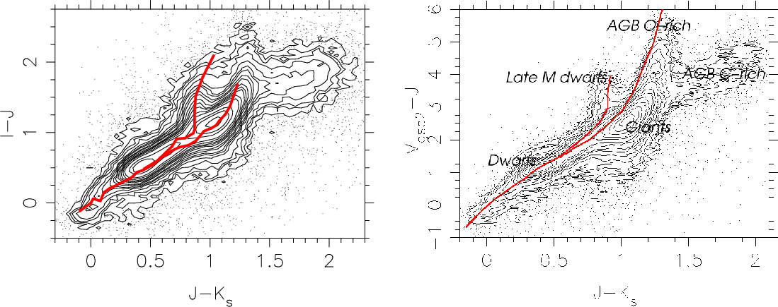Figure 13: Panel a) contains sources detected by both DCMC and 2MASS: 372 354 entries. The I band is from DENIS, whereas the J and $K_{\rm s}$ bands are from 2MASS. Dwarf and giant tracks superimposed are from Bessel & Brett (1988). Panel b) contains sources detected by both GSC2.2 and 2MASS: 147 564 entries. Dwarf and giant tracks are computed using Table 2 from Wainscoat et al. (1992). The sources involved in those diagrams have photometric errors smaller than 0.06 mag.

6.4 The ( $\mathsfsl I$, $\mathsfsl V$- $\mathsfsl K_{\mathsfsl s}$) colour-magnitude diagram

We computed several CMDs using a combination of three different wavelengths, both IR and optical, out of the different catalogues. The best features are obtained with the $V_{\rm gsc2}$, I, and $K_{\rm s}$ bands (Fig. 14).

The red supergiants (SGs) are located in the tight upward sequence at $I \sim 14$ and (V- $K_{\rm s})\sim 3$, while the blue SGs have (V- $K_{\rm s}) \leq 1$. This is consistent with the evolutionary tracks from Girardi et al. (2000). We looked at the distribution of the stars with (V- $K_{\rm s}) \leq 1$in various diagrams. The results are summarized in Fig. 15. They belong to the central parts of the LMC, and their spatial distribution is clumpy (Fig. 15d), quite similar to what Martin et al. (1976) had found with their merging of several catalogues containing SG stars. These sources are linked to the supergiant shells of the LMC (Meaburn 1980), which are probably produced by the effect of stellar winds and/or supernovae. These stars should help us constraining the recent star formation history of the LMC (Grebel & Brandner 1998; Dolphin & Hunter 1998). Some of them fall into region A of Nikolaev & Weinberg (2000) (Fig. 15a): blue SGs, O dwarfs. Since they are very blue stars, their (V-$K_{\rm s}$) colour distinguish them from the bulk of stars on the (I, V-$K_{\rm s}$) diagram (Fig. 14). They match the overdensity of stars at (I-J)=-0.25 and (J- $K_{\rm s})=0$ and extend towards redder colours (Fig. 15b). They are also recognizable on the (J-H, H-$K_{\rm s}$) diagram at (0, 0), at the bottom of the sequence of dwarfs (Fig. 15c). These young stars are much more easy to trace in the IR/optical colour-colour diagrams and CMDs than in the ($K_{\rm s}$, J-$K_{\rm s}$) CMD.