M. Rampp - H.-T. Janka
Max-Planck-Institut für Astrophysik, Karl-Schwarzschild-Str. 1, 85741 Garching, Germany
Received 8 March 2002 / Accepted 19 September 2002
Abstract
Neutrino transport and neutrino interactions
in dense matter play a crucial role in stellar
core collapse, supernova explosions and neutron star formation.
Here we present a detailed description of a new
numerical code for treating the time and energy dependent
neutrino transport in hydrodynamical simulations of such
events. The code is based on a variable Eddington
factor method to deal with the integro-differential character
of the Boltzmann equation. The moments of the neutrino distribution
function and the energy and lepton number exchange with the stellar
medium are determined by iteratively solving the zeroth and
first order moment equations in combination with a model
Boltzmann equation. The latter is discretized on a grid of
tangent rays. The integration of the transport equations and
the neutrino source terms is performed in a time-implicit way.
In the present version of the program, the transport part is
coupled to an explicit hydrodynamics code which
follows the evolution of the stellar plasma by a
finite-volume method with piecewise parabolic interpolation,
using a Riemann solver to calculate the hydrodynamic states.
The neutrino source terms are implemented in an operator-split
step. Neutrino transport and hydrodynamics can be calculated
with different spatial grids and different time steps.
The structure of the described code is modular and offers
a high degree of flexibility for an application to relativistic
and multi-dimensional problems at different levels of refinement
and accuracy. We critically evaluate results for a number of test cases,
including neutrino transport in rapidly moving stellar media and
approximate relativistic core collapse, and suggest a path for
generalizing the code to be used in multi-dimensional simulations of
convection in neutron stars and supernovae.
Key words: stars: supernovae: general - elementary particles - hydrodynamics - neutrinos
When the core of a massive star collapses to a neutron star, a huge amount of gravitational binding energy is released mainly in the form of neutrinos which are abundantly produced by particle reactions in the hot and dense plasma. In fact, the emission of neutrinos determines the sequence of dynamical events which precede the death of the star in a supernova explosion. Electron neutrinos from electron captures on protons and nuclei reduce the electron fraction and the pressure and thus accelerate the contraction of the stellar iron core to a catastrophic implosion. The position of the formation of the supernova shock at the moment of core bounce depends on the degree of deleptonization during the collapse phase. The outward propagation of the prompt shock is severely damped by energy losses due to the photodisintegration of iron nuclei, and finally stopped only a few milliseconds later when additional energy is lost in a luminous outburst of electron neutrinos. These neutrinos are created in the shock-heated matter and leave the star as soon as their diffusion is faster than the expansion of the shock. "Prompt'' supernova explosions generated by a direct propagation of the hydrodynamical shock have been obtained in simulations only when the stellar iron core is very small (Baron & Cooperstein 1990) and/or the equation of state of neutron-rich nuclear matter is extraordinarily soft (Baron et al. 1985; Baron et al. 1987).
At a later stage (roughly a hundred milliseconds after
the shock formation) the situation has changed. The
temperature behind the stalled shock has dropped such that
increasingly energetic neutrinos diffusing out from
deeper layers start to transfer energy to the stellar gas
around the nascent neutron star. If this energy deposition is
sufficiently strong, the stalled shock can be revived and a
"delayed''
explosion can be triggered (Wilson 1985; Bethe & Wilson 1985; the idea that neutrinos provide the energy of the supernova
explosion was originally brought up by Colgate & White 1966).
A small fraction of less than one per cent of the
energy released in neutrinos can account for the kinetic energy
of a typical type II supernova. This explanation is currently
favored for the explosion of massive stars in the mass range
between about 10
![]() and roughly 25
and roughly 25
![]() .
It is supported by numerical simulations and analytic
considerations. A finally convincing hydrodynamical simulation,
however, is still missing (a summary of our current
understanding of the explosion mechanism can be found
in Janka 2001). The measurement of a neutrino
signal from a Galactic supernova would offer the most direct
observational test for our theoretical perception of the onset
of the explosion. Due to the central role of neutrinos in
supernovae, the neutrino transport deserves particular
attention in numerical models.
.
It is supported by numerical simulations and analytic
considerations. A finally convincing hydrodynamical simulation,
however, is still missing (a summary of our current
understanding of the explosion mechanism can be found
in Janka 2001). The measurement of a neutrino
signal from a Galactic supernova would offer the most direct
observational test for our theoretical perception of the onset
of the explosion. Due to the central role of neutrinos in
supernovae, the neutrino transport deserves particular
attention in numerical models.
Current hydrodynamic models of neutrino-driven supernova explosions leave an ambiguous impression and have caused confusion about the status of the field outside the small community of supernova modelers. Simulations by different groups seem to be contradictory because some models show successful explosions by the neutrino-driven mechanism whereas others have found the mechanism to fail.
Wilson and collaborators have performed successful simulations for more than 15 years now (e.g., Wilson 1985; Wilson et al. 1986; Wilson & Mayle 1988; Wilson & Mayle 1993; Mayle et al. 1993; Totani et al. 1998). Their models were calculated in spherical symmetry, but shock revival was obtained by making the assumption that the neutrino luminosity is boosted by neutron-finger instabilities in the nascent neutron star (Wilson & Mayle 1988, 1993). In fact, in their calculations explosion energies comparable to typically observed values (of the order of 1051 erg) require pions to be abundant in the nuclear matter already at moderately high densities (Mayle et al. 1993). The corresponding equation of state (EoS) with pions leads to higher core temperatures and the emission of more energetic neutrinos. Both the convectively boosted luminosities and the harder spectra enhance the neutrino heating behind the stalled shock. The relevance of neutron-finger instabilities for efficient energy transport on large scales, however, has not been demonstrated by direct simulations. The existence of neutron-finger instabilities (in the sense of the definition introduced by Wilson & Mayle 1993) is indeed questioned by other investigations (Bruenn & Dineva 1996) and might be a consequence of specific properties of the high-density EoS or the treatment of the neutrino transport by Wilson and collaborators. Also the implementation of a pionic component in their EoS is at least controversial and not in agreement with other, more conventional descriptions of nuclear matter (Pethick & Pandharipande, personal communication).
Rather than finding neutron-finger instabilities, two-dimensional hydrodynamic simulations have shown that regions inside the nascent neutron star can exist where Ledoux or quasi-Ledoux convection (as defined by Wilson & Mayle 1993) develops on a time scale of tens of milliseconds after core bounce (Keil et al. 1996; Keil 1997; also Janka et al. 2001). The models were constrained to a simulation of the neutrino cooling of the nascent neutron star, but it must be expected that the convective enhancement of the neutrino luminosity, which becomes appreciable after about 200 milliseconds (see also Janka et al. 2001), can have important consequences for the revival of the stalled supernova shock (Burrows 1987). Ledoux unstable regions were also detected in spherical cooling models of newly formed neutron stars (Burrows 1987; Burrows & Lattimer 1988; Pons et al. 1999; Miralles et al. 2000). Nevertheless, their significance is controversial, because Bruenn et al. (1995) in spherically symmetric models and Mezzacappa et al. (1998a) in two-dimensional simulations observed convection inside the neutrinosphere only as a transient phenomenon during a relatively short period after core bounce.
The question is therefore undecided whether convection plays an important role in newly formed neutron stars and if so, what its implications for the supernova explosion are. Unfortunately, the various calculations were performed with different treatments of the neutrino transport, one-dimensional vs. two-dimensional hydrodynamics, general relativistic gravitational potential vs. Newtonian gravity, or even an inner boundary condition to replace the central, dense part of the neutron star core (Mezzacappa et al. 1998a). It is this inner region, however, where Keil et al. (1996) found convection to develop roughly 100 milliseconds after bounce. Convection at larger radii and thus closer below the neutrinosphere had indeed died out within only 20-30 milliseconds after shock formation in agreement with the results of Bruenn et al. (1995). Future studies with a better and more consistent handling of the different aspects of the physics are definitely needed to clarify the situation.
A second hydrodynamically unstable region develops exterior to the nascent neutron star in the neutrino-heated layer behind the stalled supernova shock. Convective overturn in this region is helpful and can lead to explosions in cases which otherwise fail (Herant et al. 1992; Herant et al. 1994; Janka & Müller 1995; Janka & Müller 1996; Burrows et al. 1995). In two-dimensional supernova models computed recently by Fryer (1999); Fryer & Heger (2000), and Fryer et al. (2002) these hydrodynamical instabilities in the postshock region are crucial for the success of the neutrino-driven mechanism, because they help transporting hot gas from the neutrino-heating region directly to the shock, while downflows simultaneously carry cold, accreted matter to the layer of strongest neutrino heating where a part of this gas readily absorbs more energy from the neutrinos. The existence of this multi-dimensional phenomenon seems to be generic for the situation which builds up in the stellar core some time after shock formation. It is therefore no matter of dispute.
All simulations showing explosions as a consequence of post-shock convection, however, have so far been performed with a strongly simplified treatment of the crucial neutrino physics, e.g., with grey, flux-limited diffusion which is matched to a "light bulb'' description at some "low'' value of the optical depth (Herant et al. 1994; Burrows et al. 1995). Alternatively, an inner boundary near the neutrinosphere had been used where the spectra and luminosities of neutrinos were prescribed to parameterize our ignorance and the potential uncertainties of the exact properties of the neutrino emission from the newly formed neutron star (Janka & Müller 1995, 1996). It is therefore not clear whether the instabilities and their associated effects in fully self-consistent and more accurate simulations will be strong enough to cause successful explosions. Doubts in that respect were raised by Mezzacappa et al. (1998b), whose two-dimensional models showed convective overturn in the neutrino-heating region but still no explosion. Mezzacappa et al. (1998b) combined two-dimensional hydrodynamics with neutrino transport results obtained by multi-group flux-limited diffusion in spherical symmetry. Although not self-consistent, their approach is nevertheless an improvement compared to previous treatments of the neutrino physics by other groups.
All computed models bear some pieces of truth. Essentially they demonstrate the remarkable sensitivity of the supernova dynamics to the different physical aspects of the problem, in particular the treatment of neutrino transport and neutrino-matter interactions, the properties of the nuclear EoS, multi-dimensional hydrodynamical processes, and general relativity. Considering the huge energy reservoir carried away by neutrinos, the neutrino-driven mechanism appears rather inefficient (the often quoted value of 1% efficiency, however, misjudges the true situation, because neutrinos can transfer between 5% and 10% of their energy to the stellar gas during the critical period of shock revival; see Janka 2001). Nevertheless, neutrino-driven explosions are "marginal'' in the sense that the energy of a standard supernova explosion is of the same order as the gravitational binding energy of the ejected progenitor mass. The final success of the supernova shock is the result of different physical processes which compete against each other. On the one hand, neutrino heating tries to drive the shock expansion, on the other hand energy losses, e.g., by neutrinos that are reemitted from the inward flow of neutrino-heated matter which enters the neutrino-cooling zone below the heating layer, extract energy and thus damp the shock revival. It is therefore not astonishing that different approximations or descriptions for one or more physical components of the problem can decide between an explosion or failure of a simulation.
None of the current supernova models includes all relevant aspects to a satisfactory level of accuracy, but all of these models are deficient in one or more respects. Wilson and collaborators obtain explosions, but their input physics is unique and cannot be considered as generally accepted. Two-dimensional (Herant et al. 1994; Burrows et al. 1995; 1999; Fryer & Heger 2000; Fryer et al. 2002) and three-dimensional (Fryer, personal communication) models show explosions due to strong postshock convection, but the neutrino transport and neutrino-matter interactions are handled at a level of accuracy which falls back behind the most elaborate treatments that have been applied in spherical symmetry. The sensitivity of the outcome of numerical calculations to details of the neutrino transport demands improvements. Self-consistent multi-dimensional simulations with a sophisticated and quantitatively reliable treatment of the neutrino physics have yet to be performed.
Most recently, spherically symmetric Newtonian (Rampp & Janka 2000; Mezzacappa et al. 2001), and general relativistic (Liebendörfer et al. 2001b) hydrodynamical simulations of stellar core-collapse and post-bounce evolution including a Boltzmann solver for the neutrino transport have become possible. Although the models do not yield explosions, they must be considered as a major achievement for the modeling of supernovae. Before these calculations only the collapse phase of the stellar core had been investigated with solving the Boltzmann equation (Mezzacappa & Bruenn 1993c). Boltzmann transport has now superseded multi-group flux-limited diffusion (Arnett 1977; Bowers & Wilson 1982; Bruenn 1985; Myra et al. 1987; Baron et al. 1989; Bruenn 1989a,b, 1993; Cooperstein & Baron 1992) as the most elaborate treatment of neutrinos in supernova models.
The differences between both methods in dynamical calculations have still to be figured out in detail, but the possibility of solving the Boltzmann equation removes imponderabilities and inaccuracies associated with the use of flux-limiters in particular in the region of semi-transparency, where neutrinos decouple from the stellar background and also deposit the energy for an explosion (Janka 1991; Janka 1992; Messer et al. 1998; Yamada et al. 1999). For the first time the transport can now be handled at a level of sophistication where the technical treatment is more accurate than our standard description of neutrino-matter interactions, which includes various approximations and simplifications (for an overview of the status of the handling of neutrino-nucleon interactions, see Horowitz 2002 and the references therein).
In this paper we describe our new numerical code for solving
the energy and time dependent
Boltzmann transport equation for neutrinos coupled to the
hydrodynamics of the stellar medium. First results
from supernova calculations with this code were published
before (Rampp & Janka 2000), but a detailed documentation of
the method will be given here. It is based on a variable
Eddington factor technique where the coupled set of Boltzmann
equation and neutrino energy and momentum equations is
iterated to convergence. Variable Eddington moments of
the neutrino phase space distribution are used for closing
the moment equations, and the integro-differential character
of the Boltzmann equation is tamed by using the zeroth and
first order angular moments (neutrino density and flux) in the
source terms on the right hand side of the Boltzmann equation.
This numerical approach is fundamentally different from the
so-called ![]() methods (Carlson 1967; Yueh & Buchler 1977; Mezzacappa & Bruenn 1993a; Yamada et al. 1999) which employ a
direct discretization of the Boltzmann equation in all variables
including the dependence on the angular direction of the
radiation propagation.
methods (Carlson 1967; Yueh & Buchler 1977; Mezzacappa & Bruenn 1993a; Yamada et al. 1999) which employ a
direct discretization of the Boltzmann equation in all variables
including the dependence on the angular direction of the
radiation propagation.
Some basic characteristics of our code are similar to elements described by Burrows et al. (2000). Different from the latter paper we shall discuss the details of the numerical implementation of the transport scheme and its coupling to a hydrodynamics code (Rampp 2000), which in our case is the PROMETHEUS code with the potential of performing multi-dimensional simulations. The variable Eddington factor technique was our method of choice for the neutrino transport because of its modularity and flexibility, which offer significant advantages for a generalization to multi-dimensional problems. We shall suggest and motivate corresponding approximations which we consider as reasonable in the supernova case, at least as a first step towards multi-dimensional hydrodynamics with a Boltzmann treatment of the neutrino transport.
This paper is arranged as follows: in Sect. 2 the equations of radiation hydrodynamics are introduced. Section 3 provides a general overview of the numerical methods used to solve these equations and contains details of their practical implementation. Results for a number of idealized test problems as well as applications of the new method to the supernova problem are presented in Sect. 4. A summary will be given in Sect. 5. In the Appendix the numerical implementation of neutrino opacities and the equation of state used for core-collapse and supernova simulations is described.
For an ideal fluid characterized by the mass density ![]() ,
the
Cartesian components of the velocity vector
,
the
Cartesian components of the velocity vector
![]() ,
the specific energy density
,
the specific energy density
![]() and
the gas pressure
p, the Eulerian, nonrelativistic equations of hydrodynamics in
Cartesian coordinates read (sum over i implied):
and
the gas pressure
p, the Eulerian, nonrelativistic equations of hydrodynamics in
Cartesian coordinates read (sum over i implied):
An equation of state is invoked in order to express the pressure as
a function of the independent thermodynamical variables,
i.e.,
![]() ,
if NSE holds, or
,
if NSE holds, or
![]() otherwise (see
Appendix B for the numerical handling of the equation of
state).
otherwise (see
Appendix B for the numerical handling of the equation of
state).
In the following we will employ spherical coordinates and, unless otherwise stated, assume spherical symmetry.
Lindquist (1966) derived a covariant transfer equation
and specialized it for particles of zero rest mass
interacting in a spherically symmetric medium supplemented with
the comoving frame metric (a is a Lagrangian coordinate)
![]() .
.
The "Lindquist-equation'', which describes the evolution
of the specific intensity ![]() as measured in the comoving frame of
reference, reads:
as measured in the comoving frame of
reference, reads:
The functional dependences of the
metric functions
![]() ,
R(t,a), the specific
intensity
,
R(t,a), the specific
intensity
![]() ,
and the collision
integral
,
and the collision
integral
![]() were suppressed for brevity.
Momentum space is described by the coordinates
were suppressed for brevity.
Momentum space is described by the coordinates ![]() and
and ![]() ,
which are the energy and the cosine of the angle of propagation
of the neutrino with respect to the radial direction, both measured in
the locally comoving frame of reference.
Note that the opacity
,
which are the energy and the cosine of the angle of propagation
of the neutrino with respect to the radial direction, both measured in
the locally comoving frame of reference.
Note that the opacity ![]() and the emissivity
and the emissivity ![]() ,
and thus the
collision integral
,
and thus the
collision integral
![]() in general depend also
explicitly on momentum-space
integrals of
in general depend also
explicitly on momentum-space
integrals of ![]() ,
which makes the transfer equation an
integro-partial differential equation.
Examples of the actual computation of the collision integral for a
number of interaction processes of neutrinos with matter can
be found in Appendix A.
,
which makes the transfer equation an
integro-partial differential equation.
Examples of the actual computation of the collision integral for a
number of interaction processes of neutrinos with matter can
be found in Appendix A.
In general, the metric functions
![]() and
R(t,a) have to be computed numerically from the Einstein
field equations.
When working to order
and
R(t,a) have to be computed numerically from the Einstein
field equations.
When working to order
![]() and in a flat
spacetime (usually called the "Newtonian approximation''), it is
however possible to express these functions analytically in terms of
only the velocity field and its first time derivative (the fluid
acceleration).
Details of the derivation can be found in Castor (1972).
Alternatively one can simply reduce the special relativistic
transfer equation (Mihalas 1980) to order
and in a flat
spacetime (usually called the "Newtonian approximation''), it is
however possible to express these functions analytically in terms of
only the velocity field and its first time derivative (the fluid
acceleration).
Details of the derivation can be found in Castor (1972).
Alternatively one can simply reduce the special relativistic
transfer equation (Mihalas 1980) to order
![]() .
.
This transfer equation, together with its
angular moment equations of zeroth and first order reads
(e.g., Mihalas & Mihalas 1984, see also Lowrie et al. 2001):
 |
(9) |
For reference we also write down the transformations
(correct to
![]() )
which allow one to relate the
frequency-integrated moments in the
comoving ("Lagrangian'') and in the inertial ("Eulerian'') frame of
reference (indicated by the superscript "Eul'').
)
which allow one to relate the
frequency-integrated moments in the
comoving ("Lagrangian'') and in the inertial ("Eulerian'') frame of
reference (indicated by the superscript "Eul'').
The system of Eqs. (6)-(8) is coupled to the
evolution equations of the
fluid (Eqs. (1)-(4)) in spherical
coordinates and symmetry) by virtue of the
definitions of the source terms
Recently, Lowrie et al. (2001) emphasized the fundamental significance
of a term
In core-collapse supernova simulations carried out so far, the dynamics of the stellar fluid presumably was not affected by neglecting the term in Eq. (6). However, our tests with Eq. (6), including the additional time derivative of Eq. (14) and the corresponding changes in the moment equations (Eqs. (7), (8)), have shown that the neutrino signal computed in a supernova simulation is indeed altered compared to the traditional treatment. We will therefore take the term of Eq. (14) into account in future simulations.
For calculating nonrelativistic problems
Mihalas & Mihalas (1984) suggested a form of the radiation momentum
equation (Eq. (8)), in which all velocity-dependent terms
except
for the
![]() -term in the first line of
Eq. (8) are dropped.
When the velocities become sizeable, however, it may be advisable
to solve the momentum equation in its general form
(Eq. (8)).
Doing so, we indeed found that the terms omitted by Mihalas & Mihalas (1984)
can have an effect on the solution of the neutrino transport in
supernovae, in particular on the neutrino energy spectrum.
-term in the first line of
Eq. (8) are dropped.
When the velocities become sizeable, however, it may be advisable
to solve the momentum equation in its general form
(Eq. (8)).
Doing so, we indeed found that the terms omitted by Mihalas & Mihalas (1984)
can have an effect on the solution of the neutrino transport in
supernovae, in particular on the neutrino energy spectrum.
For solving the neutrino radiation hydrodynamics problem we employ the well-known "operator splitting''-approach, a popular method to make large problems computationally tractable by considering them as a combination of smaller subproblems. The coupled set of equations of radiation hydrodynamics (Eqs. (1)-(4), (6)-(8)) is split into a "hydrodynamics part'' and a "neutrino part'', which are solved independently in subsequent ("fractional'') steps. In the "hydrodynamics part'' (Sect. 3.2) a solution of the equations of hydrodynamics including the effects of gravity is computed without taking into account neutrino-matter interactions.
In what we call the "neutrino part'' (Sects. 3.3-3.4) the coupled system of equations
describing the neutrino transport and
the changes of the specific internal energy e and the electron
fraction
![]() of the stellar fluid due to the emission and absorption of
neutrinos are solved. The latter changes are given by the equations
of the stellar fluid due to the emission and absorption of
neutrinos are solved. The latter changes are given by the equations
Within the neutrino part, we calculate in a first step the transport
of energy and
electron-type lepton number by neutrinos and the corresponding
exchange with the stellar fluid
for electron neutrinos (
![]() )
and antineutrinos
(
)
and antineutrinos
(
![]() )
only, which also means that the sum in
Eq. (15) is restricted to
)
only, which also means that the sum in
Eq. (15) is restricted to
![]() .
The
.
The ![]() and
and ![]() neutrinos and their antiparticles, all
represented by a single species ("
neutrinos and their antiparticles, all
represented by a single species ("![]() '') are handled together with
the remaining terms of the sum in Eq. (15) in a second
step.
'') are handled together with
the remaining terms of the sum in Eq. (15) in a second
step.
For the neutrino transport we use the so-called "variable Eddington factor'' method, which determines the neutrino phase-space distribution by iteratively solving the radiation moment equations for neutrino energy and momentum coupled to the Boltzmann transport equation. Closure of the set of moment equations is achieved by a variable Eddington factor calculated from a formal solution of the Boltzmann equation, and the integro-differential character of the latter is tamed by making use of the integral moments of the neutrino distribution as obtained from the moment equations. The method is similar to the one described by Burrows et al. (2000).
For the integration of the equations of hydrodynamics we employ the Newtonian finite-volume hydrodynamics code PROMETHEUS developed by Fryxell et al. (1989). PROMETHEUS is a direct Eulerian, time-explicit implementation of the Piecewise Parabolic Method (PPM) of Colella & Woodward (1984), which is a second-order Godunov scheme employing a Riemann solver. PROMETHEUS is particularly well suited for following discontinuities in the fluid flow like shocks or boundaries between layers of different chemical composition. It is capable of tackling multi-dimensional problems with high computational efficiency and numerical accuracy.
The version of PROMETHEUS used in our radiation hydrodynamics code was provided to us by Keil (1997). It offers an optional generalization of the Newtonian gravitational potential to include general relativistic corrections. The hydrodynamics code was considerably updated and augmented by K. Kifonidis who added a simplified version of the "Consistent Multifluid Advection (CMA)'' method (Plewa & Müller 1999) which ensures an accurate advection of the individual chemical components of the fluid. In order to avoid spurious oscillations arising in multidimensional simulations, when strong shocks are aligned with one of the coordinate lines (the so-called "odd-even decoupling'' phenomenon), a hybrid scheme was implemented (Kifonidis 2000; Plewa & Müller 2001) which, in the vicinity of such shocks, selectively switches from the original PPM method to the more diffusive HLLE solver of Einfeldt (1988).
In what follows we describe the numerical implementation of the
"Newtonian'' limit of the transport equations including
![]() -terms (cf. Sect. 2.2.2).
The general relativistic version of the code is based on almost exactly
the same considerations.
-terms (cf. Sect. 2.2.2).
The general relativistic version of the code is based on almost exactly
the same considerations.
In order to construct a conservative numerical scheme for the system of
moment equations, we integrate the moment equations
(Eqs. (7), (8)) over a zone of
the numerical
![]() -mesh.
-mesh.
After having performed the integral over the volumes ![]() of the radial mesh zones, the moment equations can be rewritten as
evolution equations for the volume-integrated moments (e.g.,
of the radial mesh zones, the moment equations can be rewritten as
evolution equations for the volume-integrated moments (e.g.,
![]() ).
In case of a moving radial grid, where the
volume
).
In case of a moving radial grid, where the
volume ![]() of a grid cell is time dependent, one has to
apply the "moving grid transport theorem'' (see e.g. Müller 1991)
in order to interchange the operators Dt and
of a grid cell is time dependent, one has to
apply the "moving grid transport theorem'' (see e.g. Müller 1991)
in order to interchange the operators Dt and
![]() .
For the special case of a Lagrangian grid,
where the grid moves with the velocity of the stellar fluid, the
latter reads:
.
For the special case of a Lagrangian grid,
where the grid moves with the velocity of the stellar fluid, the
latter reads:
The computational domain
![]() is
covered by Nr radial zones.
As the zone center
is
covered by Nr radial zones.
As the zone center
![]() we define the volume-weighted mean
of the interface coordinates ri and ri+1:
we define the volume-weighted mean
of the interface coordinates ri and ri+1:
 |
(18) |
The spectral range
![]() is covered
by a discrete energy grid consisting of
is covered
by a discrete energy grid consisting of
![]() energy "bins'',
where the centers of these zones are given in terms of the interface values as
energy "bins'',
where the centers of these zones are given in terms of the interface values as
 |
(19) |
We employ a time-implicit finite differencing scheme for the moment
equations (Eqs. (7), (8)) in combination with the
equations which describe the exchange of
internal energy and electron fraction with the stellar medium
(Eqs. (15), (16)).
Doing so we avoid the restrictive Courant Friedrichs Lewy (CFL)
condition which explicit numerical schemes have to obey for stability
reasons: for neutrino transport in the optically thin regime the CFL
condition would require
![]() ,
where
,
where
![]() is the size of the smallest zone and
is the size of the smallest zone and ![]() the
numerical time step.
Even more importantly, the time-implicit discretization allows one to
efficiently cope with the different time scales of the problem:
the "stiff'' source terms
introduce a characteristic time scale proportional to the mean free
path
the
numerical time step.
Even more importantly, the time-implicit discretization allows one to
efficiently cope with the different time scales of the problem:
the "stiff'' source terms
introduce a characteristic time scale proportional to the mean free
path ![]() of the neutrinos,
of the neutrinos,
![]() ,
which can be orders of
magnitude smaller than the CFL time step in the
opaque interior of a protoneutron star,
where the optical depth
,
which can be orders of
magnitude smaller than the CFL time step in the
opaque interior of a protoneutron star,
where the optical depth
![]() of individual grid cells becomes
very large.
of individual grid cells becomes
very large.
Applying the procedures described in Sect. 3.3.1 to the moment
equations (Eqs. (7), (8)) we obtain for each
neutrino
species
![]() (the corresponding
index is suppressed in the notation below) the finite
differenced moment equations. On an Eulerian grid they read:
(the corresponding
index is suppressed in the notation below) the finite
differenced moment equations. On an Eulerian grid they read:
Since the radiation moments are defined on a staggered mesh,
the finite-difference equations are second-order accurate in space.
First-order accuracy in time is achieved by employing fully implicit
time-differences ("backward Euler'').
Only the advection terms in the second and forth line of
Eq. (21) and Eq. (22), respectively,
are treated differently (see Sect. 4.3.1 for a motivation):
![\begin{displaymath}\iota(i):=
\left\{
\begin{array}{ll}
i-\frac{1}{2}&\quad {\rm...
...[2mm]
i+\frac{1}{2}&\quad {\rm else}~. \\
\end{array}\right.
\end{displaymath}](/articles/aa/full/2002/46/aa2451/img183.gif) |
(26) |
Using a similar diffusive term in the zeroth moment equation (Eq. (21)) allowed us also to overcome stability problems with the numerical handling of the velocity-dependent terms in the general form of the radiation momentum equation, Eq. (8).
For the solution of the moment equations (Eqs. (7),
(8)), boundary conditions have to be specified at
![]() ,
,
![]() ,
,
![]() and
and
![]() .
In the radial domain the values of quantities at the boundaries
are iteratively obtained from the solution of the Boltzmann
equation (see Sect. 3.4.3 for the boundary conditions
employed there), which has the advantage that in the moment
equations no assumptions have to be made about the angular
distribution of the specific intensity at the
boundaries.
Specifically, at the inner boundary
.
In the radial domain the values of quantities at the boundaries
are iteratively obtained from the solution of the Boltzmann
equation (see Sect. 3.4.3 for the boundary conditions
employed there), which has the advantage that in the moment
equations no assumptions have to be made about the angular
distribution of the specific intensity at the
boundaries.
Specifically, at the inner boundary
![]() is given by
is given by
![]() as computed from the Boltzmann
equation.
To handle the outer boundary, we apply Eq. (22)
on the "half shell'' between
as computed from the Boltzmann
equation.
To handle the outer boundary, we apply Eq. (22)
on the "half shell'' between
![]() and
rNr (Mihalas & Mihalas 1984). Where necessary,
and
rNr (Mihalas & Mihalas 1984). Where necessary,
![]() is
replaced by
is
replaced by
![]() in Eqs. ((21), (22)).
in Eqs. ((21), (22)).
At
![]() the flux in energy space vanishes and hence we simply
set
the flux in energy space vanishes and hence we simply
set
![]() in Eq. (21). At the upper boundary of the spectrum the flux
in energy space,
in Eq. (21). At the upper boundary of the spectrum the flux
in energy space,
![]() is computed by a
(geometrical)
extrapolation of the moments
is computed by a
(geometrical)
extrapolation of the moments
![]() and
and
![]() and by a linear extrapolation of the
advection velocity using
and by a linear extrapolation of the
advection velocity using
![]() and
and
![]() .
Analogous expressions are used for Eq. (22).
.
Analogous expressions are used for Eq. (22).
The finite differenced versions of the operator-splitted source terms
in the energy and lepton number equations (Eqs. (15),
(16)) of the stellar fluid read:
In the finite-differenced version of the (monochromatic) neutrino energy
equation (Eq. (21)) the derivative with respect to energy,
![]() ,
has been written in a conservative form.
When a summation over all energy bins is performed in
Eq. (21), the terms containing
fluxes across the boundaries of the energy zones telescope and an
appropriate finite differenced version of the total
(i.e. spectrally integrated) neutrino energy equation
is recovered.
This essential property does, however, not hold automatically also for
the neutrino number density
,
has been written in a conservative form.
When a summation over all energy bins is performed in
Eq. (21), the terms containing
fluxes across the boundaries of the energy zones telescope and an
appropriate finite differenced version of the total
(i.e. spectrally integrated) neutrino energy equation
is recovered.
This essential property does, however, not hold automatically also for
the neutrino number density
![]() ,
when the naive definition
,
when the naive definition
![]() is adopted. By inserting the latter expression into Eq. (21)
and summing over all energy bins, it can easily be verified that the
corresponding
fluxes across the boundaries of the energy bins do not cancel anymore due
to the finite cell size
is adopted. By inserting the latter expression into Eq. (21)
and summing over all energy bins, it can easily be verified that the
corresponding
fluxes across the boundaries of the energy bins do not cancel anymore due
to the finite cell size
![]() .
.
In order to avoid this problem, we instead derive the moment
equations for ![]() and
and ![]() (by multiplying
Eqs. (7), (8) with
(by multiplying
Eqs. (7), (8) with
![]() )
and
recast them into a conservative form:
)
and
recast them into a conservative form:
With the Eddington factors fH, fK, fL and flow field
![]() being given,
the nonlinear system of equations (Eqs. (21),
(22), (30), (31), (28),
(29)) is solved
for the variables
being given,
the nonlinear system of equations (Eqs. (21),
(22), (30), (31), (28),
(29)) is solved
for the variables
![]() by a Newton-Raphson iteration
(e.g. Press et al. 1992), using the aforementioned boundary conditions.
by a Newton-Raphson iteration
(e.g. Press et al. 1992), using the aforementioned boundary conditions.
This requires the inversion of a block-pentadiagonal
system with 2 Nr+1 rows of blocks. The dimension of an individual
block of the
Jacobian is
![]() in case of the transport of
electron neutrinos and antineutrinos (the number of energy bins
in case of the transport of
electron neutrinos and antineutrinos (the number of energy bins
![]() is multiplied by a factor of two because
is multiplied by a factor of two because
![]() and
and
![]() are treated as separate particles, the other factor of two
comes from the additional transport of neutrino number). In contrast,
muon and tau neutrinos and their antiparticles are considered here as
one neutrino species because their interactions with supernova matter
are roughly the same. In the absence of the corresponding charged
leptons, muon and tau neutrinos are only produced (or annihilated) as
are treated as separate particles, the other factor of two
comes from the additional transport of neutrino number). In contrast,
muon and tau neutrinos and their antiparticles are considered here as
one neutrino species because their interactions with supernova matter
are roughly the same. In the absence of the corresponding charged
leptons, muon and tau neutrinos are only produced (or annihilated) as
![]() pairs and hence do not transport lepton number.
Therefore the blocks have a dimension of
pairs and hence do not transport lepton number.
Therefore the blocks have a dimension of
![]() for these
flavours.
for these
flavours.
For setting up the Jacobian all partial derivatives with respect to the radiation moments can be calculated analytically, whereas the derivatives with respect to electron fraction and specific internal energy are approximated by finite differences.
In order to provide the closure relations (the "variable Eddington
factors'') for the truncated system of moment equations, we have to
solve the Boltzmann equation. Since the emissivity ![]() and the opacity
and the opacity ![]() depend in general also on angular moments
of
depend in general also on angular moments
of ![]() ,
this is actually a nonlinear, integro-differential
problem.
However,
,
this is actually a nonlinear, integro-differential
problem.
However, ![]() and
and ![]() become known functions of only the
coordinates t, r,
become known functions of only the
coordinates t, r, ![]() and
and ![]() ,
when
J and H are used as given solutions of the moment equations.
This allows one to calculate a formal solution of the Boltzmann
equation.
,
when
J and H are used as given solutions of the moment equations.
This allows one to calculate a formal solution of the Boltzmann
equation.
Making the change of variables
(cf. Yorke 1980; Mihalas & Mihalas 1984; Körner 1992; Basheck et al. 1997)
For the moment we shall ignore terms which contain frequency derivatives
![]() (see Eqs. (35), (36)).
These Doppler terms will be included in an operator-split manner.
(see Eqs. (35), (36)).
These Doppler terms will be included in an operator-split manner.
Equations (35), (36) are then discretized on a so-called "tangent ray grid'' (for an illustration, see Fig. 1), the geometry of which being an immediate consequence of the transformation of variables given by Eq. (32). Applying this transformation, partial derivatives of only one momentum-space coordinate s remain, whereas the second coordinate p appears only in a parametric way (cf. Baschek et al. 1997). This greatly facilitates the numerical solution of the system.
![\begin{figure}
\includegraphics[width=7.5cm,clip]{2451f1.ps}\end{figure}](/articles/aa/full/2002/46/aa2451/img244.gif) |
Figure 1:
Eulerian radial and tangent ray grid of the computation
(solid lines) and virtual Lagrangian shell at time level
|
| Open with DEXTER | |
A "tangent ray'' k is defined by its "impact parameter'' pk=rk at
![]() .
The coordinate s serves to measure
the path length along the ray.
On each tangent ray k, a staggered numerical mesh is introduced for
the coordinate s.
The zone boundaries (centers) of this mesh are given by
the ray's intersections with the zone boundaries (centers) of the
radial grid (cf. Fig. 1).
With the "flux-like'' variable h being defined at the zone boundaries
sik
and the "density-like'' variable j being defined at the zone centers
.
The coordinate s serves to measure
the path length along the ray.
On each tangent ray k, a staggered numerical mesh is introduced for
the coordinate s.
The zone boundaries (centers) of this mesh are given by
the ray's intersections with the zone boundaries (centers) of the
radial grid (cf. Fig. 1).
With the "flux-like'' variable h being defined at the zone boundaries
sik
and the "density-like'' variable j being defined at the zone centers
![]() ,
the finite-differenced versions of
Eqs. (35), (36) finally can be written down (cf. Mihalas & Klein 1982, Sect. V.2):
,
the finite-differenced versions of
Eqs. (35), (36) finally can be written down (cf. Mihalas & Klein 1982, Sect. V.2):
The frequency derivatives of Eqs. (35), (36),
which were ignored in the finite-difference versions,
Eqs. (39), (40), are
taken into account in a separate step by operator-splitting (the
partially updated values for j and h were marked by asterisks in
Eqs. (39), (40).
The discretization of the corresponding terms is explicit in time and
- provided the acceleration terms in the second line of
Eqs. (35), (36) are neglected -
can be performed straightforwardly using upwind differences in energy
space (
![]() ):
):
![\begin{displaymath}\upsilon_{i_k,k}:=
(1-\mu_{i_k,k}^2)\left[\frac{\beta}{r}\rig...
...i_k,k}^2\left[\frac{\partial\beta}{\partial r}\right]_{i_k}
~,
\end{displaymath}](/articles/aa/full/2002/46/aa2451/img261.gif) |
(44) |
It should be possible to proceed along similar lines for including the exact aberration effects in the Boltzmann solution which, for the time being, includes aberration only in an approximate way on the basis of the replacements given by Eqs. (37), (38). In practice, however, the adopted tangent-ray geometry does not allow for a conservative discretization of the angular derivatives in a way as simple as in the case of the frequency derivatives. We plan to spend extra work on the omitted angular derivatives of the intensity in order to include them in future version of our code.
On the tangent ray grid boundary conditions must be specified for
each ray k at sk,k and at sNr,k.
At the inner core radius (
![]() and
and
![]() )
we set the boundary condition
)
we set the boundary condition
![]() ,
with
,
with
![]() .
For the remaining rays (
.
For the remaining rays (
![]() ), symmetry and
Eq. (34) imply hk,k=0, since
), symmetry and
Eq. (34) imply hk,k=0, since
![]() .
.
At the outer radius
(
![]() and
and
![]() )
we consider Eq. (40) on the "half shell'' between
)
we consider Eq. (40) on the "half shell'' between
![]() and rNr (cf. Sect 3.3.3) and
make the replacement
and rNr (cf. Sect 3.3.3) and
make the replacement
![]() ,
with
,
with
![]() .
.
The physical boundary conditions are described by the functions
![]() and
and
![]() with
with
![]() ,
which specify
the specific intensity entering the computational volume at the
inner and outer surfaces, respectively.
,
which specify
the specific intensity entering the computational volume at the
inner and outer surfaces, respectively.
At the boundaries of the energy grid we use the same type of boundary conditions as described for the moment equations (cf. Sect. 3.3.3).
By virtue of the approximations used to derive the model
equations (Eqs. (35), (36)) and upon
introducing the tangent ray grid,
the system of Eqs. (39), (40) with suitably
chosen boundary conditions can be
solved independently for
each impact parameter pk, each type of neutrino (note that for
simplicity we have dropped the index ![]() in our notation), and - because Doppler shift terms are split off - each
neutrino energy bin
in our notation), and - because Doppler shift terms are split off - each
neutrino energy bin
![]() (index also suppressed).
(index also suppressed).
For the same reasons as detailed in Sect. 3.3,
we have employed fully implicit ("backward Euler'')
time differencing. Solving Eqs. (39),
(40) therefore requires the
separate solution of
![]() (
Nk:=Nr-K0+1 is the number of tangent rays)
pentadiagonal linear systems of dimension
(
Nk:=Nr-K0+1 is the number of tangent rays)
pentadiagonal linear systems of dimension ![]() Nr.
On vector computers, this can be done very
efficiently by employing a vectorization over the index k.
Once the numerical solution for j and h has been obtained,
the monochromatic angular moments and thus the Eddington factors
fH=H/J, fK=K/J and fL=L/J can be computed using the
numerical quadrature formulae
Nr.
On vector computers, this can be done very
efficiently by employing a vectorization over the index k.
Once the numerical solution for j and h has been obtained,
the monochromatic angular moments and thus the Eddington factors
fH=H/J, fK=K/J and fL=L/J can be computed using the
numerical quadrature formulae
Unless the velocity field vanishes identically (in this case
![]() and
and
![]() in Eqs. (39) and
(40), respectively),
an additional complication arises, since the partial derivative
in Eqs. (39) and
(40), respectively),
an additional complication arises, since the partial derivative
![]() has to be
evaluated not only at fixed Lagrangian radius
(the index i in our case)
but also for a fixed value of the angle cosine
has to be
evaluated not only at fixed Lagrangian radius
(the index i in our case)
but also for a fixed value of the angle cosine ![]() .
The angular grid
.
The angular grid
![]() ,
which is associated
with
the radius rin, however, changes as ri moves with time.
As a consequence, e.g., the values of h at the old
time level used in Eq. (40) are
,
which is associated
with
the radius rin, however, changes as ri moves with time.
As a consequence, e.g., the values of h at the old
time level used in Eq. (40) are
![]() and not
and not
![]() ,
the solution
of the previous time step (cf. Mihalas & Mihalas 1984, Sect. 98).
At the beginning of the time step we therefore have to interpolate
the radiation field for each fixed radial index i from
the
,
the solution
of the previous time step (cf. Mihalas & Mihalas 1984, Sect. 98).
At the beginning of the time step we therefore have to interpolate
the radiation field for each fixed radial index i from
the
![]() -grid onto the
-grid onto the
![]() -grid.
If an Eulerian grid is used for the computation,
an additional interpolation in the radial direction is
performed to map from the fixed ri-grid to the coordinates given
by
-grid.
If an Eulerian grid is used for the computation,
an additional interpolation in the radial direction is
performed to map from the fixed ri-grid to the coordinates given
by
![]() (see
Fig. 1).
This seemingly complicated procedure has the advantage of
being computationally much more efficient than directly
discretizing Eqs. (35), (36) in Eulerian
coordinates. In this case the
(see
Fig. 1).
This seemingly complicated procedure has the advantage of
being computationally much more efficient than directly
discretizing Eqs. (35), (36) in Eulerian
coordinates. In this case the
![]() -term, which
originates from making the replacement
-term, which
originates from making the replacement
![]() ,
would
couple grid points of different impact parameters and would therefore
defy an independent treatment of the tangent rays.
,
would
couple grid points of different impact parameters and would therefore
defy an independent treatment of the tangent rays.
A transport time step starts by adopting guess values (e.g., given by the
solution of the previous time step) for J, H,
![]() ,
and e.
The quantities
,
and e.
The quantities
![]() ,
e and the density
,
e and the density ![]() determine the
thermodynamic state and thus the temperature
and chemical potentials. These, together with J and H are used
to evaluate the rhs of the Boltzmann equation.
This allows one to compute its formal
solution and the Eddington factors as detailed in
Sect. 3.4.
The Eddington factors are then fed into the system of moment and
source-term equations, the solution of which (Sect. 3.3)
yields improved values for J, H,
determine the
thermodynamic state and thus the temperature
and chemical potentials. These, together with J and H are used
to evaluate the rhs of the Boltzmann equation.
This allows one to compute its formal
solution and the Eddington factors as detailed in
Sect. 3.4.
The Eddington factors are then fed into the system of moment and
source-term equations, the solution of which (Sect. 3.3)
yields improved values for J, H,
![]() ,
and e. At this point,
where required (e.g., for evaluating
,
and e. At this point,
where required (e.g., for evaluating
![]() ),
the neutrino number density
),
the neutrino number density ![]() and
number flux density
and
number flux density ![]() are conventionally replaced by
are conventionally replaced by
![]() and
and
![]() .
This procedure
is iterated until numerical convergence is achieved.
With the Eddington factors being known from the described
iteration procedure, the complete system of source-term and moment
equations for neutrino energy and number is solved (once) in
order to accomplish lepton number conservation. In this step
.
This procedure
is iterated until numerical convergence is achieved.
With the Eddington factors being known from the described
iteration procedure, the complete system of source-term and moment
equations for neutrino energy and number is solved (once) in
order to accomplish lepton number conservation. In this step
![]() and
and ![]() are treated as additional variables
(cf. Sect. 3.3.5).
are treated as additional variables
(cf. Sect. 3.3.5).
Our experience with the operator-splitting technique has shown that considerable care is necessary in how precisely the equations of hydrodynamics are coupled with the neutrino transport and how the fractional time steps are scheduled. In the following we therefore describe the used procedures in some detail.
Since the hydrodynamics code and the transport solver in general have different requirements for numerical resolution, accuracy and stability, the discretization in both space and time of the two code components is preferably chosen to be independent of each other. In supernova simulations, for example, the time step limit (from the CFL condition) for the hydrodynamic evolution computed by a time-explicit method is typically more restrictive than in the time-implicit treatment of the transport part. Since the transport is computationally much more expensive, one wants to use a larger time step than for the hydrodynamics part. This means that a transport time step is divided into a suitable number of hydrodynamical substeps.
Starting from the hydrodynamic state
![]() at the
old time level tn, the time-explicit PPM algorithm first computes a
solution of the hydrodynamical conservation laws without the
effects of gravity and neutrinos.
From the updated density, the gravitational potential can be
calculated by virtue of Poisson's equation and finally the
gravitational source
terms are applied to the total energy equation (Eq. (3))
and the momentum equation (Eq. (2)).
This completes the "hydrodynamics'' time step with size
at the
old time level tn, the time-explicit PPM algorithm first computes a
solution of the hydrodynamical conservation laws without the
effects of gravity and neutrinos.
From the updated density, the gravitational potential can be
calculated by virtue of Poisson's equation and finally the
gravitational source
terms are applied to the total energy equation (Eq. (3))
and the momentum equation (Eq. (2)).
This completes the "hydrodynamics'' time step with size
![]() ,
which is limited by the CFL-condition (see e.g., LeVeque 1992).
By performing a total of
,
which is limited by the CFL-condition (see e.g., LeVeque 1992).
By performing a total of
![]() substeps
the hydrodynamic state is evolved from the time level tn to the new
time level tn+1 given by
substeps
the hydrodynamic state is evolved from the time level tn to the new
time level tn+1 given by
 |
(49) |
After the transport time step has been completed, the new neutrino
stress
![]() is used for correcting v* to give the
new velocity vn+1 at time level tn+1:
is used for correcting v* to give the
new velocity vn+1 at time level tn+1:
![\begin{displaymath}[\rho v]^{n+1}=\rho^{n+1} v^{*}+
(Q_{\rm M}^{n+1}- Q_{\rm M}^{n})
\cdot \Delta t^n
~.
\end{displaymath}](/articles/aa/full/2002/46/aa2451/img313.gif) |
(52) |
Radial discretization of the transport and hydrodynamic equations is done on independent grids. Therefore there is freedom to choose the number of zones and their coordinate values separately in both parts of the code. Only quantities which obey conservation laws have to be communicated from the hydro to the transport grid. By invoking the equation of state all other thermodynamical quantities can be derived from the density, the total energy density, momentum density and the number densities of electrons and nuclear species. In the other direction it is the neutrino source terms which have to be mapped back onto the hydro grid.
For the mapping procedure we assume the conserved quantities to be piecewise linear functions of the radius inside the grid cells, with parameters determined by the cell average values and so-called "monotonized slopes'' (for details see, e.g., Ruffert 1992 and references cited therein). In order to achieve global conservation of integral values we then simply average this function within each cell of the target grid of the mapping (cf. Dai & Woodward 1996).
Using this procedure in dynamical supernova simulations, we discovered spurious radial and temporal fluctuations of the temperature, electron fraction, entropy and related quantities inside the opaque protoneutron star unless the hydro and transport grids coincide exactly in this region. The scale of these fluctuations is sensitive to the radial cell size and the size of a time step, the relative amplitude was found to be typically of the order of a few percent, with the exact number varying between different quantities (see Rampp & Janka 2000). These fluctuations are understood from the fact that the mapping of the source terms on the one hand and the internal energy density (resp. temperature) on the other hand implies deviations from local thermodynamical equilibrium between neutrinos and stellar medium. The attempt of the neutrino transport to restore this equilibrium within a given grid cell leads to large net production or absorption rates, driving the temperature in the opposite direction and causing it to perform oscillations in time around a mean value. Despite these oscillations and fluctuations, the use of different numerical grids inside the protoneutron star did not cause noticeable problems for the accuracy of the "global'' evolution of our models, because the conservative mapping describes the exchange of energy and lepton number between neutrinos and the stellar fluid correctly on average.
Being cautious, we take advantage of the option of using different hydro and transport grids only during the early phases of the collapse and in regions of the star, where neutrinos are far from reaching equilibrium with the stellar fluid. In this case no visible fluctuations occur.
The numerical treatment of the radiation hydrodynamics problem should guarantee that the conservation laws for energy and lepton number are fulfilled.
Provided the acceleration terms (
![]() ),
which are of order (v2/c2)and thus usually very small compared to the other terms, are ignored,
the constancy of the total lepton number is ensured by, (a) a
conservative
discretization of the neutrino number equation (Eq. (30)),
(b) a conservative handling of the electron number equation
(Eq. (4)), and (c) the exact numerical balance of the
source terms (cf. Eq. (13))
),
which are of order (v2/c2)and thus usually very small compared to the other terms, are ignored,
the constancy of the total lepton number is ensured by, (a) a
conservative
discretization of the neutrino number equation (Eq. (30)),
(b) a conservative handling of the electron number equation
(Eq. (4)), and (c) the exact numerical balance of the
source terms (cf. Eq. (13))
![]() (defined on the transport grid) and
(defined on the transport grid) and
![]() (defined on the hydro grid).
Point (a) requires that in Eq. (30) the flux divergence is
discretized in analogy to the second line in Eq. (21) and
that the
(defined on the hydro grid).
Point (a) requires that in Eq. (30) the flux divergence is
discretized in analogy to the second line in Eq. (21) and
that the
![]() and
and
![]() terms are combined to
terms are combined to
![]() to be discretized in analogy to the
third line in Eq. (21).
The energy derivative in Eq. (30) is treated in a
conservative way as described in Sect. (3.3.5).
Point (b) is achieved by the use of a conservative numerical
integration of the electron number equation
(Eq. (4)) in the spirit of the PROMETHEUS code, and
requirement (c) is fulfilled by employing a conservative
procedure for mapping the electron
number source term from the transport grid to the hydro grid (see
Sects. 3.6.1, 3.6.2).
Doing so, the total lepton number remains constant in principle at
the level of machine accuracy.
to be discretized in analogy to the
third line in Eq. (21).
The energy derivative in Eq. (30) is treated in a
conservative way as described in Sect. (3.3.5).
Point (b) is achieved by the use of a conservative numerical
integration of the electron number equation
(Eq. (4)) in the spirit of the PROMETHEUS code, and
requirement (c) is fulfilled by employing a conservative
procedure for mapping the electron
number source term from the transport grid to the hydro grid (see
Sects. 3.6.1, 3.6.2).
Doing so, the total lepton number remains constant in principle at
the level of machine accuracy.
Different from the number transport, where the zeroth order moment equation for neutrinos by itself defines a conservation law, the derivation of a conservation law for the total energy implies a combination of the radiation energy and momentum equations. The use of a staggered radial mesh for discretizing the latter equations defies a suitable contraction of terms in analogy to the analytic case. Therefore our numerical description does not conserve neutrino energy with the same accuracy as neutrino number and the quality of total energy conservation has to be verified empirically for a given problem and numerical resolution.
For our supernova simulations, tests showed that neutrino number is
conserved to an accuracy of
better than 10-11 per time step, while for neutrino energy a
value below 10-7 is achieved. With a typical
number of about 50 000 transport time steps for a supernova
simulation we thus find an empirical upper limit for the violation of
energy conservation of ![]() of the neutrino energy.
This translates to
of the neutrino energy.
This translates to ![]() of the internal energy of the
collapsed stellar core, i.e. a few times
of the internal energy of the
collapsed stellar core, i.e. a few times
![]() in
absolute number.
Errors of the same magnitude are introduced by the
non-conservative treatment of the gravitational potential as a source
term in the fluid-energy equation (Eq. (3)).
Note that the use of different grids for the hydrodynamics and the
transport does not affect the energy budget because we employ a
conservative mapping of the neutrino source term between the grids
(see
Sects. 3.6.1, 3.6.2).
in
absolute number.
Errors of the same magnitude are introduced by the
non-conservative treatment of the gravitational potential as a source
term in the fluid-energy equation (Eq. (3)).
Note that the use of different grids for the hydrodynamics and the
transport does not affect the energy budget because we employ a
conservative mapping of the neutrino source term between the grids
(see
Sects. 3.6.1, 3.6.2).
We have not yet coupled our general relativistic version of the neutrino transport to a general relativistic hydrodynamics code. For the time being we work with a basically Newtonian code, which was extended to include post-Newtonian corrections of the gravitational potential. We hope that the deeper gravitational potential can account for the main effects of general relativity on stellar core collapse and the formation of neutron stars which do not approach gravitational instability to become black holes (cf. Bruenn et al. 2001). Because the general relativistic changes of the space-time metric are ignored, a consistent description of the neutrino transport requires that the fully relativistic equations are simplified such that only the effects of gravitational redshift and time dilation are retained.
By comparing the Tolman-Oppenheimer-Volkoff equation for hydrostatic
equilibrium in general relativity (see, e.g., Kippenhahn & Weigert 1990, Sect. 2.6) with its Newtonian counterpart
(cf. Eq. (2)) one can define a modified "gravitational
potential'' which includes correction terms due to pressure and energy
of the stellar medium and the neutrinos:
Equation (53) can be used in the Newtonian hydrodynamic equations (Eqs. (2), (3)) in order to approximately take into account general relativistic effects (cf. Keil 1997). The quality of this approach has to be ascertained empirically by comparison with fully general relativistic calculations. In our case such a comparison yields quite satisfactory results (see Sect. 4.3).
The general relativistic moment equations describing transport of
neutrino energy, momentum and neutrino number can be derived from the
Lindquist-equation (cf. Eq. (5), Sect. 2.2.1).
They are:
In the approximate treatment we neglect the distinction between
coordinate radius and proper radius (
![]() ,
,
![]() )
in Eqs. (54)-(57), and
identify corresponding quantities with their Newtonian counterparts
(
)
in Eqs. (54)-(57), and
identify corresponding quantities with their Newtonian counterparts
(![]() ,
,
![]() ,
,
![]() ).
The same approximations are made in the "parent'' Boltzmann equation
from which the moment equations of the relativistic approximation can
be consistently derived.
Accordingly, the approximations to
Eqs. (54)-(57) contain only general
relativistic redshift and time dilation effects for neutrinos.
Coupling the transport with the Newtonian equations of hydrodynamics,
these restrictions to a fully relativistic treatment
are necessary in order to verify conservation
laws for energy and lepton number of the coupled system.
).
The same approximations are made in the "parent'' Boltzmann equation
from which the moment equations of the relativistic approximation can
be consistently derived.
Accordingly, the approximations to
Eqs. (54)-(57) contain only general
relativistic redshift and time dilation effects for neutrinos.
Coupling the transport with the Newtonian equations of hydrodynamics,
these restrictions to a fully relativistic treatment
are necessary in order to verify conservation
laws for energy and lepton number of the coupled system.
Finite-difference versions of the moment equations and the
corresponding parent Boltzmann equation
for the approximate GR transport are obtained by applying the techniques
described in Sects. 3.3 and 3.4.
The lapse function is calculated by integrating the general
relativistic Euler equation
![]() inward from the surface, where the boundary
condition
inward from the surface, where the boundary
condition
![]() is applied (van Riper 1979).
is applied (van Riper 1979).
Multi-dimensional frequency dependent neutrino transport in moving media and relativistic environments is a challenging problem for future work. Since convective phenomena were recognized to be highly important in supernovae (Herant et al. 1994; Burrows et al. 1995; Janka & Müller 1996; Keil et al. 1996 and refs. therein) one would of course like to perform simulations with Boltzmann neutrino transport also in two and three dimensions. Here we suggest an approximate approach based on a straightforward generalization of our variable Eddington factor method, which offers some advantages concerning computational efficiency. The approximation should be considered as an intermediate step between spherically symmetric and fully multi-dimensional models. Of course, the quality of the approximation for the neutrino transport which we will describe below, will finally have to be checked by a comparison with fully multi-dimensional transport calculations.
Our approximate treatment may be a reasonably accurate and physically justifyable approach for describing neutrino transport in situations where the star does not show a global deformation (e.g., due to rotation) in layers which are opaque to neutrinos, but where inhomogeneities and anisotropies are present only on smaller scales (e.g., due to convection). Multi-dimensional hydrodynamical simulations suggest that convective processes occur in two distinct regions of the supernova core:
Under these circumstances the specific intensity
![]() can be assumed to depend mainly on r but only weakly on longitude
can be assumed to depend mainly on r but only weakly on longitude
![]() and latitude
and latitude ![]() of the background medium.
Hence, like in the spherically
symmetric case, the dependence of the specific intensity on the direction
of propagation
of the background medium.
Hence, like in the spherically
symmetric case, the dependence of the specific intensity on the direction
of propagation ![]() can be described by only one angle
can be described by only one angle
![]() .
The flux is thus approximated as
.
The flux is thus approximated as
![]() and the scalar
and the scalar
![]() is sufficient to define the radiation stress tensor.
is sufficient to define the radiation stress tensor.
In the moment equations,
gradients in the ![]() - and the
- and the ![]() -direction, which describe
the transport of energy and neutrino number into these lateral and
azimuthal directions, are neglected, yet the parametric dependence of
the (scalar) moments on the
coordinates
-direction, which describe
the transport of energy and neutrino number into these lateral and
azimuthal directions, are neglected, yet the parametric dependence of
the (scalar) moments on the
coordinates ![]() and
and ![]() is retained and the radial
transport is computed using the moment equations independently in each
angular zone of the stellar model.
In order to close the set of moment equations, variable Eddington
factors are computed by iterating the Boltzmann equation and
the corresponding moment equations on a
spherically symmetric "image'' of the stellar
background. The latter is defined as the angular average of physical
quantities
is retained and the radial
transport is computed using the moment equations independently in each
angular zone of the stellar model.
In order to close the set of moment equations, variable Eddington
factors are computed by iterating the Boltzmann equation and
the corresponding moment equations on a
spherically symmetric "image'' of the stellar
background. The latter is defined as the angular average of physical
quantities
![]() according to
according to
![]() .
Note that the variable Eddington factors are normalized moments of the
neutrino phase space distribution function and thus should not show
significant
variation with the angular coordinates of the star. This justifies
replacing them by quantities that depend only on the radial position
and time.
.
Note that the variable Eddington factors are normalized moments of the
neutrino phase space distribution function and thus should not show
significant
variation with the angular coordinates of the star. This justifies
replacing them by quantities that depend only on the radial position
and time.
Since for each latitude ![]() and longitude
and longitude ![]() the moment
equations (Eqs. (7), (8)) in our approach are solved
together with the evolution equations of electron fraction and
internal energy due to neutrino sources (Eqs. (15),
(16), local radiative equilibrium can be attained
properly and conservation of energy can be fulfilled.
It is not obvious to us how these fundamental requirements could be
met in a more simple approximation where one uses a
one-dimensional transport scheme to compute the transport on a
spherically symmetric "mean star'', which is obtained at each time
step by averaging the multi-dimensional hydrodynamical stellar model
over angles.
the moment
equations (Eqs. (7), (8)) in our approach are solved
together with the evolution equations of electron fraction and
internal energy due to neutrino sources (Eqs. (15),
(16), local radiative equilibrium can be attained
properly and conservation of energy can be fulfilled.
It is not obvious to us how these fundamental requirements could be
met in a more simple approximation where one uses a
one-dimensional transport scheme to compute the transport on a
spherically symmetric "mean star'', which is obtained at each time
step by averaging the multi-dimensional hydrodynamical stellar model
over angles.
Besides having significant advantages for easy and efficient
implementation on vector and parallel computer architectures, the
suggested approach also saves computer time compared to a multiple
application of a one-dimensional Boltzmann solver.
Let
![]() be the computation time required for
calculating a time step of the full one-dimensional transport problem
and let
be the computation time required for
calculating a time step of the full one-dimensional transport problem
and let
![]() be the number of steps that are
necessary for the iteration between the moment equations and the
Boltzmann equation to achieve convergence.
If
be the number of steps that are
necessary for the iteration between the moment equations and the
Boltzmann equation to achieve convergence.
If
![]() is the total
number of angular zones that discretize the background star, the
computation time for calculating one time step of the
multi-dimensional problem with the described approximate method is
is the total
number of angular zones that discretize the background star, the
computation time for calculating one time step of the
multi-dimensional problem with the described approximate method is
 |
(58) |
 |
(59) |
Stationary solutions of the Boltzmann equation of radiative transfer can be calculated analytically, semi-analytically or numerically to high accuracy in a few cases, where a particularly simple form of the emissivity and the opacity is assumed. These problems provide test cases for our new code for solving the equations of neutrino transport. To this end we impose suitably chosen initial and boundary conditions and solve the time-dependent neutrino transport equations numerically, until a stationary state is reached. The numerical solutions can then be compared to the reference solutions. This first class of problems, presented in Sects. 4.1 and 4.2, does neither refer to specific properties of neutrinos nor will the equations of neutrino radiation hydrodynamics, i.e. the coupling of the neutrino transport equation to the equations of hydrodynamics, be tested. Time-dependent hydrodynamical tests will be described in Sect. 4.3.
We first consider the simplest class of radiative transfer problems, namely those where the "background medium'' is assumed to be time-independent and static, i.e. the radial profiles of the emissivity and opacity do not change with time and the velocity and acceleration vanish everywhere and at all times. As usual, the background medium is assumed to be spherically symmetric.
Here, our method for computing the variable Eddington
factor (see Sect. 3.4) by solving the Boltzmann
equation with a finite difference scheme (Mihalas & Klein 1982)
is compared with results obtained from a
general quadrature solution along characteristics (Yorke 1980; Körner 1992; Baschek et al. 1997).
For convenience, we set ![]() in this section.
in this section.
As a test problem we consider a central point source which emits
radiation with an intensity
![]() into a spherical, static and homogeneous
shell of matter bounded by two spheres of radius r0 and R > r0.
The only interaction of the radiation with the medium is by
absorption (
into a spherical, static and homogeneous
shell of matter bounded by two spheres of radius r0 and R > r0.
The only interaction of the radiation with the medium is by
absorption (
![]() ).
The central source is active during the time interval
).
The central source is active during the time interval
![]() .
Initially (t=0), there is no radiation inside the shell.
.
Initially (t=0), there is no radiation inside the shell.
By symmetry, the intensity vanishes for all but the radial
direction of propagation. In the absence of scattering,
it is therefore sufficient to follow the propagation of the light pulse
along a single radial (characteristic) ray. The dependence of
the intensity on the angle can thus conveniently be
suppressed in the notation, writing
| (60) |
 |
(63) |
Figure 2 shows our results for
![]() at the time
t=100, together with the analytical solution (Eq. (63)).
We define the position of the numerically broadened light
front as the radius, where the average of the true
pre and postfront value of the intensity is reached.
In all cases the mean propagation speed is well reproduced, with
some minor loss of accuracy for very large time steps.
The shape of the light front, however, deviates from the true
solution. One observes an artificial precursor together with
a reduced intensity behind the front,
both effects resulting in a spatial broadening of the front.
A clear trend towards larger diffusive broadening with increasing
time steps can be seen from Fig. 2 and
Table 1. This phenomenon was also observed by
Mihalas & Klein (1982), who reported very similar results for their tests.
at the time
t=100, together with the analytical solution (Eq. (63)).
We define the position of the numerically broadened light
front as the radius, where the average of the true
pre and postfront value of the intensity is reached.
In all cases the mean propagation speed is well reproduced, with
some minor loss of accuracy for very large time steps.
The shape of the light front, however, deviates from the true
solution. One observes an artificial precursor together with
a reduced intensity behind the front,
both effects resulting in a spatial broadening of the front.
A clear trend towards larger diffusive broadening with increasing
time steps can be seen from Fig. 2 and
Table 1. This phenomenon was also observed by
Mihalas & Klein (1982), who reported very similar results for their tests.
Table 1 summarizes our results for the width of the front
and compares them to
simulations done with an implementation of the method of characteristics
(Yorke 1980; Körner 1992).
The latter method has the advantage to exactly reproduce the
analytical solution without any smearing of the front, if the
light front is advanced by exactly one grid cell per time step.
Though the ability to reproduce the exact solution appears to be a
very appealing property of the method of characteristics,
the necessary condition
![]() can hardly ever be
accomplished in realistic simulations. This is simply due to the fact
that in typical astrophysical simulations the radial resolution can be
varying over several orders of magnitude, whereas in most
applications the global value of the time step is determined in
some region of the grid.
When doing radiation hydrodynamical simulations, for example, one is usually
interested in resolving time scales different from those
given by the speed of propagating light fronts.
Accordingly, the time steps can be very different from the optimum for
describing the light front propagation.
Our finite difference scheme therefore seems to be preferable to the
method of characteristics as far as the resolution of travelling
discontinuities is concerned (cf. Table 1).
can hardly ever be
accomplished in realistic simulations. This is simply due to the fact
that in typical astrophysical simulations the radial resolution can be
varying over several orders of magnitude, whereas in most
applications the global value of the time step is determined in
some region of the grid.
When doing radiation hydrodynamical simulations, for example, one is usually
interested in resolving time scales different from those
given by the speed of propagating light fronts.
Accordingly, the time steps can be very different from the optimum for
describing the light front propagation.
Our finite difference scheme therefore seems to be preferable to the
method of characteristics as far as the resolution of travelling
discontinuities is concerned (cf. Table 1).
![\begin{figure}
\includegraphics[width=12.5cm,clip]{2451f2.eps}\end{figure}](/articles/aa/full/2002/46/aa2451/img397.gif) |
Figure 2:
Outwardly directed intensity
|
| Open with DEXTER | |
For time steps ![]() significantly smaller than the
radial zone width, a case not discussed by Mihalas & Klein (1982), we
observe some spurious postfront oscillations
(see also Mihalas & Weaver 1982, Sect. 5) .
Their maximum amplitude, however, does not
grow with time, which is in agreement with a local von Neumann
stability analysis for the fully implicit implementation of the equations
(Mihalas & Klein 1982).
If present in practical applications, the oscillations can be damped
by employing an additional diffusive term in Eq. (62),
which is active in nearly transparent regions
(
significantly smaller than the
radial zone width, a case not discussed by Mihalas & Klein (1982), we
observe some spurious postfront oscillations
(see also Mihalas & Weaver 1982, Sect. 5) .
Their maximum amplitude, however, does not
grow with time, which is in agreement with a local von Neumann
stability analysis for the fully implicit implementation of the equations
(Mihalas & Klein 1982).
If present in practical applications, the oscillations can be damped
by employing an additional diffusive term in Eq. (62),
which is active in nearly transparent regions
(
![]() )
of the computational grid
(cf. Sects. 3.3.2, 3.4.2; Blinnikov et al. 1998).
Due to the correspondingly increased diffusivity of the
finite-difference scheme
the light front is smeared over a larger number of zones (
)
of the computational grid
(cf. Sects. 3.3.2, 3.4.2; Blinnikov et al. 1998).
Due to the correspondingly increased diffusivity of the
finite-difference scheme
the light front is smeared over a larger number of zones (
![]() for
for
![]() ;
see also the inserted panel in
Fig. 2a) as compared to the original method
of Mihalas & Klein (1982). Note, however, that the representation of the
front is still better than the results obtained with the method of
characteristics.
;
see also the inserted panel in
Fig. 2a) as compared to the original method
of Mihalas & Klein (1982). Note, however, that the representation of the
front is still better than the results obtained with the method of
characteristics.
| model VAC | model ABS | ||||
|
|
# | ||||
| 0.02 | 5000 | 6 | 25 | 6 | 26 |
| 0.1 | 1000 | 8 | - | 8 | - |
| 0.5 | 200 | 18 | 16 | 16 | 20 |
| 1.0 | 100 | 26 | 1 | 22 | 1 |
| 2.0 | 50 | 37 | 26 | 29 | 26 |
| 10.0 | 10 | 80 | - | 55 | - |
The so-called "homogeneous sphere'' is a test problem frequently employed for radiative transfer calculations (e.g., Bruenn 1985; Schinder & Bludman 1989; Smit et al. 1997). Physically, one can think of a static, homogeneous and isothermal sphere of radius R radiating into vacuum. Inside the sphere, the only interactions of the radiation with the background medium are isotropic absorption and thermal emission of radiation.
Despite of its simplification, the model has some important numerical and physical properties which are typically found in practical applications: Finite difference methods are challenged by the discontinuity at the surface of the sphere. Moreover, the sudden transition from radiation diffusion inside an optically thick sphere to free streaming in the ambient vacuum - a similar but less extreme situation arises in the neutrino-heating region of a core-collapse supernova - is a major source of inaccuracies for approximate radiative transfer methods like, e.g., flux-limited diffusion.
The model is defined by setting
![]() with
with
![]() ,
,
![]() for
for
![]() ,
and
,
and
![]() for r > R.
Since for this choice of parameters, the right hand side of the
Boltzmann equation does not contain terms that depend
explicitly on the angular moments of the radiation field, the solution
of Eq. (6), with
for r > R.
Since for this choice of parameters, the right hand side of the
Boltzmann equation does not contain terms that depend
explicitly on the angular moments of the radiation field, the solution
of Eq. (6), with
![]() ,
can be obtained
analytically by computing a formal solution.
With the boundary conditions
,
can be obtained
analytically by computing a formal solution.
With the boundary conditions
![]() and
and
![]() ,
which account for
isotropy (due to spherical symmetry) of the radiation field at
the center and no incoming radiation at the outer boundary,
respectively, the result for the stationary state
is (see e.g., Smit et al. 1997):
,
which account for
isotropy (due to spherical symmetry) of the radiation field at
the center and no incoming radiation at the outer boundary,
respectively, the result for the stationary state
is (see e.g., Smit et al. 1997):
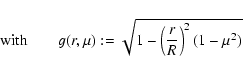 |
(65) |
We employ a radial grid consisting of 213 radial zones to cover the range
between r=0 and
![]() .
Approximately 200 zones were distributed logarithmically between
.
Approximately 200 zones were distributed logarithmically between
![]() and
and
![]() ,
about two thirds of which were spent to resolve the sphere.
Initially we set
,
about two thirds of which were spent to resolve the sphere.
Initially we set
![]() everywhere and evolved the
radiation field until a stationary state was reached.
everywhere and evolved the
radiation field until a stationary state was reached.
![\begin{figure}
\includegraphics[width=12.5cm,clip]{2451f3.eps}\end{figure}](/articles/aa/full/2002/46/aa2451/img418.gif) |
Figure 3:
Numerical (dotted and dash-dotted lines) and analytical
(solid lines) stationary-state solutions vs. radius (normalized to
the radius
|
| Open with DEXTER | |
In Fig. 3 we display the stationary-state solutions for two
models, one with ![]() (Figs. 3a, c) and another with
(Figs. 3a, c) and another with
![]() (Figs. 3b, d), representative of spheres with low
and high optical depth, respectively.
In general, our numerical results agree very well
with the analytical solutions.
The Eddington factor K/J (as calculated from the
Boltzmann equation) and the flux factor H/J (as obtained from the
moment equations) both follow the exact values very
closely (Figs. 3c, d), in case of the flux factor over many
orders of magnitude.
In both models, the transition to
free streaming is reproduced very accurately (Figs. 3c, d).
This region usually causes serious problems for flux-limited
diffusion methods (see e.g., Bruenn 1985; Smit et al. 1997).
Also the forward peaking of the radiation distribution at large
distances from the
surface of the sphere (cf. Eqs. (64), (65)) is
described excellently by our method:
at
(Figs. 3b, d), representative of spheres with low
and high optical depth, respectively.
In general, our numerical results agree very well
with the analytical solutions.
The Eddington factor K/J (as calculated from the
Boltzmann equation) and the flux factor H/J (as obtained from the
moment equations) both follow the exact values very
closely (Figs. 3c, d), in case of the flux factor over many
orders of magnitude.
In both models, the transition to
free streaming is reproduced very accurately (Figs. 3c, d).
This region usually causes serious problems for flux-limited
diffusion methods (see e.g., Bruenn 1985; Smit et al. 1997).
Also the forward peaking of the radiation distribution at large
distances from the
surface of the sphere (cf. Eqs. (64), (65)) is
described excellently by our method:
at
![]() ,
the tangent ray grid
yields approximately 150 angular grid points to resolve the radiation
field from the central source, which has an opening half angle of
only
,
the tangent ray grid
yields approximately 150 angular grid points to resolve the radiation
field from the central source, which has an opening half angle of
only
![]() (
(
![]() ).
These numbers should be compared with calculations employing the
discrete angles (
).
These numbers should be compared with calculations employing the
discrete angles (
![]() )
method: In time dependent neutrino
transport calculations, typically less than 10 angular
grid points can be afforded to equidistantly cover the range
)
method: In time dependent neutrino
transport calculations, typically less than 10 angular
grid points can be afforded to equidistantly cover the range
![]() .
.
Although we have used a geometrical
radial zoning for our tangent-ray grid, we do not find any systematic
effects caused by a "bias'' in angular binning as described by
Burrows et al. (2000).
Far from a central source, they report Eddington factors and flux
factors that asymptote to between 0.96 and 0.98 instead of 1.0 in this
case.
For example, we find values of
K/J=0.996602
for the Eddington factor and
H/J=0.999361 for the flux factor
at
![]() (in the model with
(in the model with ![]() ), to be
compared with
K/J=0.996636 and
H/J=0.998626 obtained from the
analytical solution (Eqs. (64), (4.1)).
), to be
compared with
K/J=0.996636 and
H/J=0.998626 obtained from the
analytical solution (Eqs. (64), (4.1)).
In case of the mean intensity J we observe a systematic trend towards
larger deviations from the true solution for spheres with larger total
optical depth ![]() .
In our "low opacity'' case (
.
In our "low opacity'' case (![]() ,
see Fig. 3a), there
is hardly any difference visible, whereas in the "high opacity'' case
(
,
see Fig. 3a), there
is hardly any difference visible, whereas in the "high opacity'' case
(![]() ,
see Fig. 3b) the numerical solution slightly
overestimates the true solution in a narrow region beneath the surface
of the sphere and underestimates it in the ambient vacuum region. A
detailed analysis of the data yields values of
,
see Fig. 3b) the numerical solution slightly
overestimates the true solution in a narrow region beneath the surface
of the sphere and underestimates it in the ambient vacuum region. A
detailed analysis of the data yields values of ![]() and
and ![]() for
the relative deviations from the analytical solutions in the "low
opacity'' and the "high opacity'' case, respectively.
for
the relative deviations from the analytical solutions in the "low
opacity'' and the "high opacity'' case, respectively.
This finding is caused by the steep opacity gradient near the surface
of the radiating sphere. Since we keep our radial grid to be the same
in all models, the transition from high optical depth
(
![]() ,
if r<R) to transparency
(
,
if r<R) to transparency
(![]() ,
if r>R) occurs in a boundary layer beneath the surface
of the sphere, which is less well resolved when the opacity is very
large.
In the "high opacity''
case, the semi-transparent layer is geometrically much thinner than
in the "low opacity'' case and therefore the radial gradients of the
radiation density are steeper and would require more radial zones for
a proper description.
In fact, in the "low opacity'' case the radial zones of our grid
near the surface of the sphere are optically thin (
,
if r>R) occurs in a boundary layer beneath the surface
of the sphere, which is less well resolved when the opacity is very
large.
In the "high opacity''
case, the semi-transparent layer is geometrically much thinner than
in the "low opacity'' case and therefore the radial gradients of the
radiation density are steeper and would require more radial zones for
a proper description.
In fact, in the "low opacity'' case the radial zones of our grid
near the surface of the sphere are optically thin (
![]() ), whereas in the "high opacity'' case the outermost
zone has already an optical depth of
), whereas in the "high opacity'' case the outermost
zone has already an optical depth of
![]() .
A better quality of the numerical results could be achieved by
increasing the spatial resolution in
the vicinity of large opacity or emissivity gradients and/or by
using higher-order difference schemes.
.
A better quality of the numerical results could be achieved by
increasing the spatial resolution in
the vicinity of large opacity or emissivity gradients and/or by
using higher-order difference schemes.
Due to the absence of scattering in the discussion of the homogeneous sphere problem, the solution of the Boltzmann equation does not require any information from the moment equations. No iteration between both parts of the code is necessary. Therefore this problem allows one to test the algorithm which solves the Boltzmann equation for the radiation intensity independently from the numerical solution of the moment equations. For the stationary state, we find that the radiation moments calculated by a numerical integration of the intensities are consistent with the moments directly obtained from the moment equations to within an accuracy of less than a percent.
Hummer & Rybicki (1971) published stationary-state solutions for the
spherical analogue of the classical Milne problem.
The model comprises a static, spherically symmetric, pure scattering
atmosphere of some radius
![]() ,
with a central point source
that is emitting radiation isotropically with a constant luminosity
L0.
Due to the presence of scattering, the problem is of
integro-differential nature and defies solution by
simply computing the formal solution of the Boltzmann equation.
,
with a central point source
that is emitting radiation isotropically with a constant luminosity
L0.
Due to the presence of scattering, the problem is of
integro-differential nature and defies solution by
simply computing the formal solution of the Boltzmann equation.
The opacity of the atmosphere is assumed to be solely caused by isotropic
scattering with a simple power-law dependence on radius:
For a number of atmospheres defined by various combinations of the
parameters
![]() ,
,
![]() and
and
![]() ,
Hummer & Rybicki (1971) computed numerically the zeroth moment J
and the Eddington factor K/J of the stationary-state solution as a
function of radius.
They found values of better than one percent for the accuracy of their
results.
The stationary-state solution for the first moment H as a function
of radius can easily be derived analytically from the zeroth order
moment equation (Eq. (7), with
,
Hummer & Rybicki (1971) computed numerically the zeroth moment J
and the Eddington factor K/J of the stationary-state solution as a
function of radius.
They found values of better than one percent for the accuracy of their
results.
The stationary-state solution for the first moment H as a function
of radius can easily be derived analytically from the zeroth order
moment equation (Eq. (7), with
![]() ):
):
The idealized concept of a central point source with a given luminosity
L0 is in practice modeled by imposing a suitable inner boundary
condition at some finite radius
![]() ,
which bounds the
atmosphere from below.
Since all atmospheres with a scattering opacity according to
Eq. (66) become optically thick at sufficiently small
radius, it is reasonable to employ the diffusion ansatz
,
which bounds the
atmosphere from below.
Since all atmospheres with a scattering opacity according to
Eq. (66) become optically thick at sufficiently small
radius, it is reasonable to employ the diffusion ansatz
We evolved the transport to stationary-state solutions for the two
sets of parameter combinations
(n=1.5,
![]() ,
,
![]() ),
and (n=2,
),
and (n=2,
![]() ,
,
![]() ).
The total optical depth at
).
The total optical depth at
![]() is larger than
55 for all models of the former class (n=1.5) and larger than
90 for all of
the models with n=2. Hence, we verify that the inner boundary is
placed at
a radius which is sufficiently small to justify the use of the
diffusion approximation (Eq. (68)) for the inner boundary
condition.
In order to test the sensitivity of the results to the corresponding angular dependence of the
intensity (Eq. (68)), we have calculated a model
with a different angular dependence:
is larger than
55 for all models of the former class (n=1.5) and larger than
90 for all of
the models with n=2. Hence, we verify that the inner boundary is
placed at
a radius which is sufficiently small to justify the use of the
diffusion approximation (Eq. (68)) for the inner boundary
condition.
In order to test the sensitivity of the results to the corresponding angular dependence of the
intensity (Eq. (68)), we have calculated a model
with a different angular dependence:
![]() .
The parameter
.
The parameter
![]() is chosen such that
is chosen such that
![]() .
This prescription is appropriate for an
atmosphere around a central hollow sphere with radius
.
This prescription is appropriate for an
atmosphere around a central hollow sphere with radius
![]() ,
which is irradiated from below by the central point source.
Figure 4d shows the Eddington factor of the stationary
state for this model.
The numerical solution deviates visibly from the reference solution
only in the innermost radial zones.
,
which is irradiated from below by the central point source.
Figure 4d shows the Eddington factor of the stationary
state for this model.
The numerical solution deviates visibly from the reference solution
only in the innermost radial zones.
![\begin{figure}
\includegraphics[width=12.5cm,clip]{2451f4.eps}\end{figure}](/articles/aa/full/2002/46/aa2451/img456.gif) |
Figure 4:
Stationary state solutions for selected radiation
quantities as a function of radius obtained
with our radiative transfer code (solid lines). Our results are
compared with the reference solutions (crosses) and asymptotic
solutions (dashed lines) of Hummer & Rybicki (1971).
Panel a): mean intensity J (times r2) for the combination
of model parameters
|
| Open with DEXTER | |
In the models with n=1.5 the standard radial grid consisted of 200 logarithmically distributed zones with some additional zones giving higher resolution near the surface of the atmosphere, whereas 250 equidistant radial zones were used for the models with n=2. Additional tests with 500 radial grid points were performed for some selected models without finding significant changes. Figure 4 shows some results of our tests together with the data of Hummer & Rybicki (1971). The agreement is excellent. In all models we were able to reproduce the analytical solution for the flux (Eq. (67)) with a relative accuracy of at least 10-4 throughout the atmosphere.
![\begin{figure}
\includegraphics[width=12.5cm,clip]{2451f5.eps}\end{figure}](/articles/aa/full/2002/46/aa2451/img457.gif) |
Figure 5:
Metric functions |
| Open with DEXTER | |
Schinder & Bludman (1989) considered the effects of a strong gravitational field
in some of the radiative transfer problems discussed above, in
particular in the cases of a homogeneous sphere and a static
scattering atmosphere.
They computed stationary-state solutions numerically for the
general relativistic equations of radiative transfer and compared the
results to the weak field limit.
For a static background (
![]() ),
and by application of a change of coordinates
),
and by application of a change of coordinates
![]() ,
Schinder & Bludman (1989) simplified the general relativistic moment equations
(Eqs. (54), (55)) to
,
Schinder & Bludman (1989) simplified the general relativistic moment equations
(Eqs. (54), (55)) to
Different from the moment equations, which we treat in their most general form (Eqs. (54), (55)), our implementation of the tangent ray scheme for computing the variable Eddington factors employs a number of approximations. In particular, by using straight lines for the tangent rays, general relativistic ray bending is not included. The current tests therefore serve the purpose of clarifying the influence of these approximations on the quality of the solutions of the moment equations. Schinder & Bludman (1989) found significant differences of the Eddington factors for the general relativistic and Newtonian simulations of the scattering atmosphere (while in case of the homogeneous sphere the differences were minor). The scattering atmospheres therefore seems to be an ideal test case for our purposes.
Following Schinder & Bludman (1989),
we choose the parameters
![]() and
n=2. The variation of the metric functions
and
n=2. The variation of the metric functions
![]() and
and
![]() with radius is depicted in Fig. 5a.
All other model parameters like boundary conditions and initial
conditions are the same as in the "weak-field''-case which is defined
by
with radius is depicted in Fig. 5a.
All other model parameters like boundary conditions and initial
conditions are the same as in the "weak-field''-case which is defined
by
![]() (see above).
The stationary-state Eddington factor as computed from the Boltzmann
equation in our program is displayed as a function of
radius in Fig. 5c. The deviation from the
relativistically correct results of Schinder & Bludman (1989) is significant.
On the other hand, our result is very close to the corresponding
"weak-field'' case, which is not shown in Fig. 5.
This indicates that general relativistic ray bending, which is not
correctly taken into account in our calculation, has a determining
influence on the Eddington factor, while
the contraction of rods and time dilation - both included in our
calculation of the Eddington factor - are of minor importance.
Indeed, the relativistically correct characteristic curves
deviate considerably from straight rays, as can be seen
in Schinder & Bludman (1989, Fig. 9).
(see above).
The stationary-state Eddington factor as computed from the Boltzmann
equation in our program is displayed as a function of
radius in Fig. 5c. The deviation from the
relativistically correct results of Schinder & Bludman (1989) is significant.
On the other hand, our result is very close to the corresponding
"weak-field'' case, which is not shown in Fig. 5.
This indicates that general relativistic ray bending, which is not
correctly taken into account in our calculation, has a determining
influence on the Eddington factor, while
the contraction of rods and time dilation - both included in our
calculation of the Eddington factor - are of minor importance.
Indeed, the relativistically correct characteristic curves
deviate considerably from straight rays, as can be seen
in Schinder & Bludman (1989, Fig. 9).
The analytical stationary-state solution for the radiation flux density,
which is easily verified![]() to read
to read
![]() ,
(with
,
(with
![]() ), is reproduced with an
accuracy of 10-7.
This, of course, was to be expected for the atmosphere with
isoenergetic scattering,
since in the stationary state, the solution H(r) is
solely determined by the zeroth moment equation (Eq. (69))
with no reference to the (incorrect) Eddington factor.
), is reproduced with an
accuracy of 10-7.
This, of course, was to be expected for the atmosphere with
isoenergetic scattering,
since in the stationary state, the solution H(r) is
solely determined by the zeroth moment equation (Eq. (69))
with no reference to the (incorrect) Eddington factor.
More remarkably, the quality of our solution for
the mean intensity J(r), which is governed in the stationary
state by Eq. (70) and thus
is directly influenced by the Eddington factor, appears to be rather
good, too.
As can be seen from Fig. 5b,
the slope of the general relativistic result is reproduced correctly
throughout the atmosphere.
The quantitative agreement is quite satisfactory as well.
In judging the accuracy of our results one has to keep in mind that
the model computed here is a rather extreme case in two respects:
Firstly, the deviations of the metric functions
![]() and
and
![]() from unity (see Fig. 5a) are larger
than those typically encountered in supernova simulations when the
neutron star is not going to collapse to a black hole.
Secondly, as stated in the beginning, the effect of a curved spacetime
on the radiation field was observed by Schinder & Bludman (1989) to be much
larger for the scattering atmosphere than in a case dominated by
absorption (and emission). We expect real situations to be somewhere
in between these two extremes.
from unity (see Fig. 5a) are larger
than those typically encountered in supernova simulations when the
neutron star is not going to collapse to a black hole.
Secondly, as stated in the beginning, the effect of a curved spacetime
on the radiation field was observed by Schinder & Bludman (1989) to be much
larger for the scattering atmosphere than in a case dominated by
absorption (and emission). We expect real situations to be somewhere
in between these two extremes.
![\begin{figure}
\includegraphics[width=12.5cm,clip]{2451f6.eps} \end{figure}](/articles/aa/full/2002/46/aa2451/img471.gif) |
Figure 6:
Stationary-state angular mean J (times
r2) of the intensity as measured in the comoving frame of
reference. The abscissa gives the radial position. Results are
shown for gray scattering
atmospheres that expand according to a linear (Model "LVL'';
Panel a) and the quadratic (Model "QVL'';
Panel b) velocity law.
The thin vertical line marks the upper boundary of the atmospheres.
Different line styles of the curves correspond to different values
of the parameter
|
| Open with DEXTER | |
In the following section we consider radiative transfer problems in moving,
yet stationary background media. This means that in addition to
time-independent radial profiles of the opacity and emissivity,
a time-independent velocity field as a function of radius is prescribed.
Stationary-state solutions for the radiation field are expected to
exist is such cases and have been computed to high accuracy for
some test problems including differentially moving atmospheres with
relativistic velocities.
By comparison with fully (special) relativistic calculations, we are not
only able to
test our implementation of the velocity dependent terms but can also
judge the quality of the employed
![]() -approximation of
special relativistic effects in the equations of radiative transfer.
-approximation of
special relativistic effects in the equations of radiative transfer.
Upon introducing a non-vanishing velocity field a particular frame has
to be specified, where physical quantities are measured. In all cases
considered in this work, the latter is chosen to be the Lagrangian or
comoving frame of reference. This has to be distinguished from
the (numerical) coordinate grid that is used to simply label the
events in spacetime. Although the
transformation between different coordinate grids is trivial from an
analytical point of view (e.g., the simple replacement
![]() transforms from Eulerian
to Lagrangian coordinates), the numerical
treatment can be involved (cf. Sect. 3.4, where our
algorithm for computing a formal solution of the radiative transfer
equation in Eulerian coordinates is described).
Therefore we present test results obtained with two different
versions of our radiative-transfer code, one which uses
Lagrangian coordinates and another one which employs an Eulerian
coordinate grid.
transforms from Eulerian
to Lagrangian coordinates), the numerical
treatment can be involved (cf. Sect. 3.4, where our
algorithm for computing a formal solution of the radiative transfer
equation in Eulerian coordinates is described).
Therefore we present test results obtained with two different
versions of our radiative-transfer code, one which uses
Lagrangian coordinates and another one which employs an Eulerian
coordinate grid.
![\begin{figure}
\includegraphics[width=12.5cm,clip]{2451f7.eps}\end{figure}](/articles/aa/full/2002/46/aa2451/img473.gif) |
Figure 7:
Frequency integrated zeroth order angular moment of the
comoving frame
intensity (
|
| Open with DEXTER | |
Mihalas (1980) presents stationary-state solutions for the same type of purely scattering atmospheres considered above. In addition to the static case, he investigated differentially expanding atmospheres with relativistic velocities.
We refer to this paper and study two classes of atmospheres as test
problems, which differ in the functional dependence of the expansion
velocity (
![]() )
on the radius:
)
on the radius:
The scattering opacity of the expanding atmospheres is the same
as the one used for the static cases in
Sect. 4.1 except for the unit of length, which,
for the ease of comparison, is adopted from Mihalas (1980):
For our simulations we used a numerical grid with 200 radial
points, which were initially distributed logarithmically between
![]() and
and
![]() .
Following Mihalas (1980) as closely as possible,
we impose the boundary conditions
.
Following Mihalas (1980) as closely as possible,
we impose the boundary conditions
| = | |||
| = | (73) |
We compare our stationary-state solutions with results obtained by
Mihalas (1980). In the latter investigation a numerical method that is
accurate to all orders in v/c was
employed to solve the stationary radiative transfer equation.
We therefore do not only test the correct numerical implementation of
the
![]() equations (Eqs. (6)-(8)),
but we can also get a feeling for the quality of the
equations (Eqs. (6)-(8)),
but we can also get a feeling for the quality of the
![]() -approximation to the special relativistic transfer
equation.
All characteristic features
of the solution, discussed in detail by Mihalas (1980), are reproduced
correctly by our implementation of the
-approximation to the special relativistic transfer
equation.
All characteristic features
of the solution, discussed in detail by Mihalas (1980), are reproduced
correctly by our implementation of the
![]() equations.
It is remarkable how accurately the fully relativistic solutions are
reproduced (Fig. 6). The differences are
equations.
It is remarkable how accurately the fully relativistic solutions are
reproduced (Fig. 6). The differences are ![]() 10%,
even for
10%,
even for
![]() .
.
![\begin{figure}
\includegraphics[width=12.5cm,clip]{2451f8.eps}\end{figure}](/articles/aa/full/2002/46/aa2451/img495.gif) |
Figure 8:
Spectral distributions of the angular moment J of the
comoving frame intensity for our
stationary-state solutions of the
|
| Open with DEXTER | |
Mihalas (1980) computed stationary-state solutions also for relativistically expanding nongray atmospheres, i.e., the opacity and emissivity depended explicitly on the radiation frequency. Therefore the full frequency dependence of the comoving frame Boltzmann equation had to be retained. The atmospheres were assumed to be stationary, to emit a thermal continuum of radiation, and to be isothermal, i.e., no radial or temporal variations of the source function were present. The radiation-matter interaction was solely via absorption and emission.
Introducing the dimensionless "frequency''
![]() (the
temperature T is measured in units of the Boltzmann constant
(the
temperature T is measured in units of the Boltzmann constant
![]() ),
the emissivity reads
),
the emissivity reads
Following Mihalas (1980),
we consider the two examples (1) ![]() ,
,
![]() ,
and (2)
,
and (2)
![]() ,
,
![]() .
In the former case the frequency
.
In the former case the frequency ![]() ,
where the opacity jump is located, is considerably larger than the
frequency of the maximum of the Planck function
(
,
where the opacity jump is located, is considerably larger than the
frequency of the maximum of the Planck function
(
![]() ),
whereas it is close to the maximum in the latter case.
),
whereas it is close to the maximum in the latter case.
The radial extent of the atmospheres was chosen to be
![]() in both cases. For all models the linear
law (m=1, cf. Eq. (71)) for the expansion
velocity as a function of radius was used.
The results presented below were obtained using an Eulerian
coordinate grid. Our code version with a Lagrangian grid yields very
similar results.
in both cases. For all models the linear
law (m=1, cf. Eq. (71)) for the expansion
velocity as a function of radius was used.
The results presented below were obtained using an Eulerian
coordinate grid. Our code version with a Lagrangian grid yields very
similar results.
We have used 200 logarithmically distributed radial zones for the
radial range
![]() ,
supplemented by a few additional
zones between
,
supplemented by a few additional
zones between
![]() .
Boundary conditions were chosen as usual: Spherical symmetry at the
coordinate center requires
.
Boundary conditions were chosen as usual: Spherical symmetry at the
coordinate center requires
![]() ,
and demanding that no
radiation is entering through the surface of the atmosphere translates to
the condition
,
and demanding that no
radiation is entering through the surface of the atmosphere translates to
the condition
![]() .
.
The energy grid consisted of 21 bins (very similar results were
obtained using 8 and 12 bins instead) of equal width covering the
range
![]() for Model (1) and
for Model (1) and
![]() for Model (2), respectively.
Details about the stationary-state solutions
and their physical interpretation can be found in Mihalas (1980, Sect. 5).
In our test calculations we were able to reproduce all qualitative
trends discussed there.
The quantitative agreement of the zeroth order angular moment J of the
specific intensity is within a few percent
(see Fig. 7),
even for the case of
for Model (2), respectively.
Details about the stationary-state solutions
and their physical interpretation can be found in Mihalas (1980, Sect. 5).
In our test calculations we were able to reproduce all qualitative
trends discussed there.
The quantitative agreement of the zeroth order angular moment J of the
specific intensity is within a few percent
(see Fig. 7),
even for the case of
![]() .
This, as previously stated, does not only demonstrate the accuracy of
our numerical implementation
but even more importantly also justifies the physical
approximations employed in the underlying finite difference equations.
Note that in applications of our code to supernova calculations, one
expects velocities that are not in excess of
.
This, as previously stated, does not only demonstrate the accuracy of
our numerical implementation
but even more importantly also justifies the physical
approximations employed in the underlying finite difference equations.
Note that in applications of our code to supernova calculations, one
expects velocities that are not in excess of
![]() .
.
A rigorous comparison of the spectral distribution of the
angular moment J as calculated by our radiative transfer code
(cf. Fig. 8) with the results of Mihalas (1980) is
difficult, since he shows only results for the
static case and the rather extreme case
![]() .
The latter atmosphere obviously cannot be modeled reasonably well
with our
.
The latter atmosphere obviously cannot be modeled reasonably well
with our
![]() -code.
Nevertheless, by inspection of Figs. 3 and 4 of Mihalas (1980) one can
infer that the shapes of our spectra as displayed in
Fig. 8 exhibit the correct qualitative dependence on the
expansion velocity.
-code.
Nevertheless, by inspection of Figs. 3 and 4 of Mihalas (1980) one can
infer that the shapes of our spectra as displayed in
Fig. 8 exhibit the correct qualitative dependence on the
expansion velocity.
As an important consistency check we verified that, to order
![]() ,
the numerical solution of our implementation of the
comoving frame equations shows the correct transformation properties of
the stress-energy tensor of radiation (see Eq. (10))
and no unphysical artifacts are caused by the choice of a moving
reference frame (cf. the critique of Lowrie et al. 1999).
,
the numerical solution of our implementation of the
comoving frame equations shows the correct transformation properties of
the stress-energy tensor of radiation (see Eq. (10))
and no unphysical artifacts are caused by the choice of a moving
reference frame (cf. the critique of Lowrie et al. 1999).
For this purpose results are produced for neutrino transport in a
thermally and hydrodynamically frozen post-bounce model of
a supernova calculation by Bruenn (1993). This model can be characterized
as follows:
Neutrinos are emitted from a hot and dense hydrostatic inner core with
a radius of
![]() km.
This inner core is surrounded by a supersonically infalling outer core,
which is effectively transparent to the radiation.
Velocities in this outer atmosphere range from
km.
This inner core is surrounded by a supersonically infalling outer core,
which is effectively transparent to the radiation.
Velocities in this outer atmosphere range from
![]() to
to
![]() .
.
The stress-energy tensor as derived from the stationary-state solution of the comoving frame transport equation (Eq. (6)) is transformed to the Eulerian frame (i.e. the inertial frame in which the center of the star is at rest) and can then be compared with the result of an independent calculation which solves the transport equation directly in the Eulerian frame.
![\begin{figure}
\includegraphics[width=12.5cm,clip]{2451f9.eps}\end{figure}](/articles/aa/full/2002/46/aa2451/img521.gif) |
Figure 9:
Comparison of the stationary-state solutions of the comoving
frame transfer equation (bold lines) with the solutions after
transformation to
the Eulerian frame (thin lines) and a reference calculation for a
static stellar background ( |
| Open with DEXTER | |
Figure 9 shows the components
![]() and
and
![]() of the
stress-energy tensor (scaled by r2 c and r2, respectively).
Due to the large inwardly
directed velocities in the outer atmosphere, the neutrinos emitted by
the inner core are blueshifted for observers which
are locally comoving with the fluid flow (see the bold
lines in Fig. 9).
When the stress-energy tensor is transformed to the
Eulerian frame (Eq. (10)), this effect obviously
disappears (thin lines in Fig. 9).
Comparison with the stress-energy tensor obtained by solving the
transport equation directly in the Eulerian frame
(dashed lines in Fig. 9) reveals good agreement for both
the energy density E and the energy
flux density F in the rapidly moving atmosphere. This demonstrates
that no unphysical frame dependence is present in the calculations.
The fluctuations of the transformed energy flux density near the
center are caused by the term
of the
stress-energy tensor (scaled by r2 c and r2, respectively).
Due to the large inwardly
directed velocities in the outer atmosphere, the neutrinos emitted by
the inner core are blueshifted for observers which
are locally comoving with the fluid flow (see the bold
lines in Fig. 9).
When the stress-energy tensor is transformed to the
Eulerian frame (Eq. (10)), this effect obviously
disappears (thin lines in Fig. 9).
Comparison with the stress-energy tensor obtained by solving the
transport equation directly in the Eulerian frame
(dashed lines in Fig. 9) reveals good agreement for both
the energy density E and the energy
flux density F in the rapidly moving atmosphere. This demonstrates
that no unphysical frame dependence is present in the calculations.
The fluctuations of the transformed energy flux density near the
center are caused by the term
![]() in the expression for
in the expression for
![]() in Eq. (10). Because J (and K)
are large compared with H in the dense interior, even small
velocities lead to a significant "advective contribution'' to
in Eq. (10). Because J (and K)
are large compared with H in the dense interior, even small
velocities lead to a significant "advective contribution'' to
![]() .
.
Note that an Eulerian-frame calculation in general requires complicated velocity-dependent transformations of the source terms on the rhs of the transport equation (see Mihalas & Mihalas 1984). This, however, is unnecessary in the specific situation of the discussed model: Because the region where most of the neutrinos are produced moves with low velocities, the source terms there can be evaluated in the rest frame of the fluid. In the outer atmosphere on the other hand, where the large velocities would require a careful transformation, the source terms nearly vanish. This allowed us to simply drop the velocity-dependent terms on the lhs of Eq. (6) in order to perform a calculation with results that are in agreement with the Eulerian frame solution in the low-density part of the star.
Our new neutrino hydrodynamics code has already been applied to
dynamical supernova simulations (Rampp & Janka 2000).
Here we report some results of a Newtonian calculation of the
collapse phase of a stellar iron core with mass
![]() (plus the innermost
(plus the innermost
![]() of the silicon shell).
It is the core of a
of the silicon shell).
It is the core of a
![]() progenitor
star (Model "s15s7b2'', Woosley 1999; Heger 2000).
We compare the results to a calculation published by Bruenn & Mezzacappa (1997).
The input physics, in particular the stellar model and the
high-density equation of state, were adopted from
model "B'' of Bruenn & Mezzacappa (1997), with the exception that we do
not include neutrinos other than
progenitor
star (Model "s15s7b2'', Woosley 1999; Heger 2000).
We compare the results to a calculation published by Bruenn & Mezzacappa (1997).
The input physics, in particular the stellar model and the
high-density equation of state, were adopted from
model "B'' of Bruenn & Mezzacappa (1997), with the exception that we do
not include neutrinos other than
![]() .
This,
however, does not make a difference during the collapse phase where the
electron degeneracy is so high that only
.
This,
however, does not make a difference during the collapse phase where the
electron degeneracy is so high that only
![]() can be produced in
significant numbers.
can be produced in
significant numbers.
![\begin{figure}
\par\includegraphics[width=9cm,clip]{2451f10.eps}\end{figure}](/articles/aa/full/2002/46/aa2451/img528.gif) |
Figure 10:
Profiles of the total lepton fraction
|
| Open with DEXTER | |
The hydrodynamics was solved on a grid with 400 radial zones out to 20 000 km, which were moved with the infalling matter during core collapse. For the transport we used an Eulerian grid with 213 geometrically spaced radial zones, 233 tangent rays and 21 energy bins geometrically distributed between 0 and 380 MeV the center of the first zone being at 2 MeV.
![\begin{figure}
\includegraphics[width=10cm,clip]{2451f11.ps}\end{figure}](/articles/aa/full/2002/46/aa2451/img529.gif) |
Figure 11:
Central lepton fraction
|
| Open with DEXTER | |
The total lepton fraction
![]() and the entropy per baryon at the center of the core as a function of
the central density are displayed in Fig. 11.
The agreement with results of Bruenn & Mezzacappa (1997) is excellent.
Also the total lepton fraction as a function of enclosed mass matches
perfectly (Fig. 10).
Defining the shock formation point according to Bruenn & Mezzacappa (1997) as
the mass coordinate where the entropy per baryon after
core bounce first reaches a value of
and the entropy per baryon at the center of the core as a function of
the central density are displayed in Fig. 11.
The agreement with results of Bruenn & Mezzacappa (1997) is excellent.
Also the total lepton fraction as a function of enclosed mass matches
perfectly (Fig. 10).
Defining the shock formation point according to Bruenn & Mezzacappa (1997) as
the mass coordinate where the entropy per baryon after
core bounce first reaches a value of
![]() we find
we find
![]() .
This is about
.
This is about
![]() or 5%
larger than the value given by Bruenn & Mezzacappa (1997, Table V).
or 5%
larger than the value given by Bruenn & Mezzacappa (1997, Table V).
Judging our results, one should, of course, take into account
that Bruenn & Mezzacappa (1997) employed
a multi-group flux-limited diffusion (MGFLD) approximation for treating
the neutrino transport, whereas our code solves the Boltzmann equation.
Mezzacappa & Bruenn (1993b,c) performed a detailed comparison of
core-collapse simulations with MGFLD and with their Boltzmann solver
based on the
![]() -method.
For the quantities presented here they also found good agreement of
their results throughout the inner core.
-method.
For the quantities presented here they also found good agreement of
their results throughout the inner core.
In the outer regions of the collapsing core, the situation is somewhat
different:
Mezzacappa & Bruenn (1993b,c) demonstrated that a
number of quantities reveal significant deviations between
MGFLD and the Boltzmann transport (
![]() -method).
In particular, they obtained an electron neutrino
fraction which was by up to 20% larger in the Boltzmann run.
For the total lepton fraction, however, the difference was only 1%.
Our results (Fig. 10) confirm the agreement of Boltzmann and
MGFLD results for the latter quantity.
A more detailed comparison between the variable
Eddington factor method and the
-method).
In particular, they obtained an electron neutrino
fraction which was by up to 20% larger in the Boltzmann run.
For the total lepton fraction, however, the difference was only 1%.
Our results (Fig. 10) confirm the agreement of Boltzmann and
MGFLD results for the latter quantity.
A more detailed comparison between the variable
Eddington factor method and the
![]() -method,
however, is desirable and currently underway.
-method,
however, is desirable and currently underway.
![\begin{figure}
\includegraphics[width=12.5cm,clip]{2451f12.eps}\end{figure}](/articles/aa/full/2002/46/aa2451/img535.gif) |
Figure 12:
Electron neutrino fraction
|
| Open with DEXTER | |
A few quantities exhibit spurious oscillations as a function of the
radial (mass-) coordinate and time in our core-collapse simulations.
Figure 12a shows such features for
the electron neutrino fraction in the mass shells
![]() when the central density is
when the central density is
![]()
![]() .
Similar structures are visible in the profile of the entropy per
baryon and in the neutrino luminosity as a function of radius (or
mass) once the central density becomes larger than
.
Similar structures are visible in the profile of the entropy per
baryon and in the neutrino luminosity as a function of radius (or
mass) once the central density becomes larger than
![]()
![]() .
They can also be seen in the
central entropy as a function of the central density or time
(cf. Fig. 11b).
Mezzacappa & Bruenn (1993c) found a similar effect in their
core-collapse calculations. They identified the finite
spectral resolution of the degenerate Fermi distribution of the
electron neutrinos
to be the origin of these oscillations (Mezzacappa & Bruenn 1993c, Sect. 3.3).
.
They can also be seen in the
central entropy as a function of the central density or time
(cf. Fig. 11b).
Mezzacappa & Bruenn (1993c) found a similar effect in their
core-collapse calculations. They identified the finite
spectral resolution of the degenerate Fermi distribution of the
electron neutrinos
to be the origin of these oscillations (Mezzacappa & Bruenn 1993c, Sect. 3.3).
For comparison, we have computed a collapse model with a significantly improved spectral resolution: instead of 21 bins we used 81 energy zones to describe the energy spectrum between 0 and 380 MeV. A result of this simulation is displayed in Fig. 12b. The neutrino fraction (and related quantities) are now perfectly smooth functions of the mass coordinate.
A reasonable compromise between accuracy and computational load could be achieved by using approximately 20-30 (geometrically spaced) energy bins. This seems to be sufficient to adequately treat the sharp Fermi surface of the degenerate distribution of electron neutrinos that builds up during collapse. Even for less energy bins fluctuating quantities follow the correct evolutionary trends (Fig. 12a). Therefore we conclude with the remark that the presence of oscillations in some transport quantities may be considered as undesirable. The overall evolution of the collapsing core, its deleptonization or the shock formation radius, however, were found not to be sensitive to such "noise''.
Also during the post-bounce evolution (for which the transport of
![]() was included), we determined no significant differences
between the dynamical evolution of a model with 17 energy bins and
a model computed with 27 energy bins, using an otherwise identical
setup: At a
time of 100 ms after bounce, the structure of the models, measured by
the radial positions of fluid elements with the same mass coordinate,
agreed within a relative error of <1%.
This is corroborated by the fact that
for given snapshots from the dynamical evolution we found the neutrino
source terms
was included), we determined no significant differences
between the dynamical evolution of a model with 17 energy bins and
a model computed with 27 energy bins, using an otherwise identical
setup: At a
time of 100 ms after bounce, the structure of the models, measured by
the radial positions of fluid elements with the same mass coordinate,
agreed within a relative error of <1%.
This is corroborated by the fact that
for given snapshots from the dynamical evolution we found the neutrino
source terms
![]() and also
and also ![]() to be practically identical
in both calculations.
to be practically identical
in both calculations.
Varying the number of radial zones for the hydrodynamic and transport
parts of the code between 100 and 200 and using a comoving
hydrodynamic grid during the phase of stellar core collapse, we found
no significant changes of the results. The same holds true for the
post-bounce evolution where we switch to a fixed, Eulerian grid.
The only exception to this insensitivity is the central density at
bounce, which shows variations of up to ![]() ,
depending on the size
of the innermost zones of the hydrodynamic grid.
,
depending on the size
of the innermost zones of the hydrodynamic grid.
The choice of the radial grid, however, also influences the size of the numerical time step. According to our experience the latter has to be chosen very carefully. We give two examples here:
We also tried to assess the quality of our approximate treatment of
general
relativity (GR) in the equations of hydrodynamics and neutrino transport
(cf. Sect. 3.7).
For this purpose we performed core-collapse
simulations for the
![]() progenitor star "s15s7b2'' and
compared characteristic quantities with the information given for a MGFLD
simulation of the same star in a recent paper by Bruenn et al. (2001), and
for a Boltzmann simulation by Liebendörfer et al. (2001a).
progenitor star "s15s7b2'' and
compared characteristic quantities with the information given for a MGFLD
simulation of the same star in a recent paper by Bruenn et al. (2001), and
for a Boltzmann simulation by Liebendörfer et al. (2001a).
For the hydrodynamics we used 400 radial zones out to 10 000 km, which were moved with the infalling matter during core collapse. The transport was solved on an Eulerian grid with 200 geometrically spaced radial zones, 220 tangent rays and 17 energy bins geometrically distributed between 0 and 380 MeV the center of the first zone being at 2 MeV.
At bounce, which occurs at
![]() (
(
![]() )
after the start of the calculation, the central density reaches a
maximum of
)
after the start of the calculation, the central density reaches a
maximum of
![]()
![]() (
(
![]()
![]() )
in our GR
model (for comparison, the corresponding values for the Newtonian runs
are given in brackets). The hydrodynamic shock forms at a mass
coordinate of
)
in our GR
model (for comparison, the corresponding values for the Newtonian runs
are given in brackets). The hydrodynamic shock forms at a mass
coordinate of
![]() (
(
![]() ).
For the same stellar model, Bruenn et al. (2001) found a bounce density of
).
For the same stellar model, Bruenn et al. (2001) found a bounce density of
![]()
![]() for the general
relativistic simulation
(
for the general
relativistic simulation
(
![]()
![]() ).
The corresponding time of the bounce was
).
The corresponding time of the bounce was
![]() (
(
![]() ).
Liebendörfer et al. (2001a) located the shock formation at a mass coordinate of
).
Liebendörfer et al. (2001a) located the shock formation at a mass coordinate of
![]() (
(
![]() ).
).
Since the collapse time is determined by the slow initial phase of the
contraction, which is sensitive to the
initial conditions and the details of the numerical treatment at the
start of the calculation (Liebendörfer, personal communication),
it may be better to use the difference between the GR and the
Newtonian simulations, instead of comparing absolute times at bounce.
Our value of
![]() is very
close to the result of Bruenn et al. (2001):
is very
close to the result of Bruenn et al. (2001):
![]() .
A part of the remaining difference may be attributed to the fact
that Bruenn et al. (2001) employed a MGFLD
approximation of the neutrino transport with some smaller
differences also in the input physics (e.g., Bruenn et al. 2001 as
well as Liebendörfer et al. 2001a did not take into account ion-ion correlations for the
coherent scattering, but we did).
.
A part of the remaining difference may be attributed to the fact
that Bruenn et al. (2001) employed a MGFLD
approximation of the neutrino transport with some smaller
differences also in the input physics (e.g., Bruenn et al. 2001 as
well as Liebendörfer et al. 2001a did not take into account ion-ion correlations for the
coherent scattering, but we did).
At the level of comparison which is possible on grounds of published numbers we conclude that the agreement between our approximate treatment of GR and the relativistic core collapse seems to be reasonably good.
We have presented a detailed description of the numerical implementation of our new neutrino transport code and its coupling to a hydrodynamics program which allows simulations in spherical symmetry as well as in two or three dimensions. The transport code solves the energy and time dependent Boltzmann equation by a variable Eddington factor technique. To this end a model Boltzmann equation is discretized along tangent rays and integrated for determining the variable Eddington factors which provide the closure relations for the moment equations of neutrino energy and momentum. The latter yield updated values of the neutrino energy density and neutrino flux, which are fed back into the Boltzmann equation to handle the collision integral on its right hand side.
The system of Boltzmann equation and moment equations together with the operator-splitted terms of lepton number and energy exchange with the stellar background (which influence the evolution of the thermodynamical quantities and the composition of the stellar medium and thus the neutrino-matter interactions) are iterated to convergence. Lepton number conservation is ensured by solving additional moment equations for neutrino number density and number flux.
The integration is performed with implicit time stepping, which avoids rigorous limitations by the CFL condition and ensures that equilibrium between neutrinos and stellar medium can be established accurately and without oscillations despite of stiff neutrino absorption and emission terms. The coupling of energy bins due to Doppler shifts and energy changing scattering processes is implemented in a fully implicit way. When coupling the transport part to an explicit hydrodynamics program, as done in this work, computational efficiency requires to have the option of using different time step lengths for transport and hydrodynamics. In addition, we found it advantageous to have implemented the possibility of choosing different radial grids for both components of the program, and to switch between Lagrangian and Eulerian coordinates dependent on the considered physical problem (although we always measure physical quantities of the transport in the comoving frame of reference).
We have suggested an approximation for applying the code to multi-dimensional supernova simulations which can account for the fact that hydrodynamically unstable layers develop in the collapsed stellar core. The variable Eddington factor method offers the advantage that this can be done numerically rather efficiently (concerning programming effort as well as computational load). Although the neutrino moment equations for the radial transport are solved independently in all angular zones of the spherical grid of the multi-dimensional hydrodynamical simulation, the set of moment equations is closed by a variable Eddington factor which is computed only once for an angularly averaged stellar background.
This approximation saves a significant amount of computer time compared to truely multi-dimensional transport, and yields a code structure which can easily be implemented on parallel computers. The treatment is constrained to radial transport and thus neglects lateral propagation of neutrinos. Its applicability is therefore limited to physical problems where no global asphericities occur. It must also be considered just as a first, approximate step towards a really multi-dimensional transport in convective layers inside the neutrinosphere. The approach, however, should be perfectly suitable to treat anisotropies associated with convective overturn in the neutrino-heated region between the neutron star and the supernova shock. In the latter region neutrinos are only loosely coupled to the stellar medium (the optical depth is typically only 0.05-0.2). Therefore the energy and lepton number exchange between neutrinos and the stellar medium depends on the presence of anisotropies and inhomogeneities, whereas the transport of neutrinos is essentially unaffected by non-radial motions of the stellar plasma.
In preliminary multi-dimensional simulations of transport in convecting neutron stars we have convinced ourselves that this method guarantees good numerical convergence, because the variable Eddington factor as a normalized quantity depends only weakly on lateral variations in the stellar medium. The method ensures global energy conservation and enables local thermodynamical equilibrium between stellar medium and neutrinos to be established when the optical depth is sufficiently high. We therefore think that the proposed approximation is practicable for neutrino transport in multi-dimensional supernova simulations before fully multi-dimensional transport becomes feasible. The latter is certainly a major challenge for the years to come.
Our transport code exists in a
![]() version for
nonrelativistically moving media, and in a general relativistic
version. We have not yet coupled it to a hydrodynamics
program in full general relativity. Instead, we performed
calculations of approximate relativistic core collapse, where
corrections to the Newtonian gravitational potential were included and
only the redshift and time dilation effects were retained in the
transport equations (this means that space-time is considered
to be flat). The results for stellar core collapse compared
with published fully relativistic calculations
(with Boltzmann neutrino transport by Liebendörfer et
al. 2001 and with multi-group flux-limited diffusion by
Bruenn et al. 2001) are
encouraging and suggest that this approximation works
reasonably well and accounts for the most important effects
of relativistic gravity as long as one does not get very
close to the limit of black hole formation.
version for
nonrelativistically moving media, and in a general relativistic
version. We have not yet coupled it to a hydrodynamics
program in full general relativity. Instead, we performed
calculations of approximate relativistic core collapse, where
corrections to the Newtonian gravitational potential were included and
only the redshift and time dilation effects were retained in the
transport equations (this means that space-time is considered
to be flat). The results for stellar core collapse compared
with published fully relativistic calculations
(with Boltzmann neutrino transport by Liebendörfer et
al. 2001 and with multi-group flux-limited diffusion by
Bruenn et al. 2001) are
encouraging and suggest that this approximation works
reasonably well and accounts for the most important effects
of relativistic gravity as long as one does not get very
close to the limit of black hole formation.
We have presented results for a variety of idealized, partly
analytically solvable test calculations (in spherical
symmetry) which demonstrate the
numerical efficiency and accuracy of our neutrino transport
code. The "neutrino radiation hydrodynamics'' was verified
by core-collapse and post-bounce simulations for cases where
published results were available and could reasonably well
serve for a comparison
(a direct and more detailed comparion with Boltzmann
calculations using the ![]() method by
M. Liebendörfer and A. Mezzacappa is in progress).
method by
M. Liebendörfer and A. Mezzacappa is in progress).
Tests for a number of static model atmospheres showed that
the treatment of the angular dependence of the neutrino
transport and phase space distribution can be
handled accurately by the variable Eddington factor method.
This holds for moderately strong general relativistic
problems, too, even if ray bending effects are neglected in
the determination of the variable Eddington factor.
The numerical quality of the handling of the energy dependence
of the transport was also checked by considering background
models with stationary fluid flow. We included a model with
mildly relativistic motion (up to v/c = 0.5) and found
that the code produces accurate and physically
consistent results although we employ
an
![]() approximation to the special relativistic,
comoving frame radiative transfer equation. Also the omission
of some velocity-dependent terms in the model Boltzmann
equation for determining the variable Eddington factor
turned out not to be harmful in this respect. Closing the
radiation moment equations by a variable Eddington factor
seems to be remarkably robust against approximations in the
treatment of the Boltzmann equation.
approximation to the special relativistic,
comoving frame radiative transfer equation. Also the omission
of some velocity-dependent terms in the model Boltzmann
equation for determining the variable Eddington factor
turned out not to be harmful in this respect. Closing the
radiation moment equations by a variable Eddington factor
seems to be remarkably robust against approximations in the
treatment of the Boltzmann equation.
The tests have also demonstrated that our code performs very efficiently. Only a few iterations (typically between 3 and 7) are needed for obtaining a converged solution of the system of Boltzmann equation and moment equations even in cases where scattering rates dominate neutrino absorption. The calculation of the formal solution of the Boltzmann equation, from which the variable Eddington factor is derived, turned out to consume only 10-20% of the computer time. The major computational load comes from the inversion of the set of moment equations. The latter have a reduced dimensionality relative to the Boltzmann equation, because the dependence on the angular direction of the radiation propagation was removed by carrying out the angular integration. This advantage, however, has to be payed for by the iteration procedure with the Boltzmann equation.
Using Boltzmann solvers for the neutrino transport means a new level of sophistication in hydrodynamical simulations of supernova core collapse and post-bounce evolution. It permits a technical handling of the transport which for the first time is more accurate than the standard treatment of neutrino-matter interactions. The latter includes a number of approximations and simplifications which should be replaced by a better description, for example the detailed reaction kinematics of neutrino-nucleon interactions, phase space blocking of nucleons, effects due to weak magnetism in neutrino-nucleon reactions, or nucleon correlations in the dense medium of the neutron star (Reddy et al. 1998; Reddy et al. 1999; Burrows & Sawyer 1999; Horowitz 2002).
Boltzmann calculations will not only remove imponderabilities associated with the use of approximate methods for the neutrino transport in hydrodynamical supernova models. They will also allow for much more reliable predictions of the temporal, spectral and flavour properties of the neutrino signal from supernovae and newly formed neutron stars. This is an indispensable requirement for the interpretation of a future measurement of neutrinos from a Galactic supernova.
Acknowledgements
We thank our referee, A. Mezzacappa, for insightful comments which helped us improving the original manuscript. We are grateful to K. Kifonidis, T. Plewa and E. Müller for the latest version of the PROMETHEUS code, to K. Kifonidis for contributing a matrix solver for the transport on parallel computer platforms, and to R. Buras for implementing the three-flavour version of the code and coining subroutines to calculate the neutrino pair and bremsstrahlung rates. We thank S. Bruenn, R. Fischer, W. Keil, M. Liebendörfer and G. Raffelt for helpful conversations, and M. Liebendörfer for providing us with data of his simulations. The Institute for Nuclear Theory at the University of Washington is gratefully acknowledged for its hospitality and the Department of Energy for support during a visit of the Summer Program on Neutron Stars. This work was also supported by the Sonderforschungsbereich 375 on "Astroparticle Physics'' of the Deutsche Forschungsgemeinschaft. The computations were performed on the NEC SX-5/3C of the Rechenzentrum Garching and on the CRAY T90 of the John von Neumann Institute for Computing (NIC) in Jülich.
In this appendix we shall describe the neutrino-matter interactions
that are included in the current version of our neutrino transport
code for supernova simulations. We shall focus on aspects which are
specific and important for their numerical handling and will present
final rate expressions in the form used in our code and with a
consistent notation.
| Reaction | Rate described in | Reference | ||
|
|
|
|
Sects. A.1.2, A.2.4 | Mezzacappa & Bruenn (1993b); Cernohorsky (1994) |
|
|
|
|
Sects. A.1.2, A.2.3 | Horowitz (1997); Bruenn & Mezzacappa (1997) |
|
|
|
|
Sects. A.1.2, A.2.1 | Bruenn (1985); Mezzacappa & Bruenn (1993c) |
|
|
|
|
Sects. A.1.1, A.2.1 | Bruenn (1985); Mezzacappa & Bruenn (1993c) |
|
|
|
|
Sects. A.1.1, A.2.1 | Bruenn (1985); Mezzacappa & Bruenn (1993c) |
|
|
|
|
Sects. A.1.1, A.2.2 | Bruenn (1985); Mezzacappa & Bruenn (1993c) |
|
|
|
|
Sects. A.1.3, A.2.5 | Bruenn (1985); Pons et al. (1998) |
|
|
|
|
Sects. A.1.3, A.2.6 | Hannestad & Raffelt (1998) |
In the following we discuss the different neutrino-matter interaction
processes which contribute to the source term
("collision integral'') on the rhs of the Boltzmann
equation:
The rate of change (modulo a factor of 1/c) of the neutrino
distribution function due to absorption and emission processes
is given by (see Bruenn 1985)
The rate of change of the neutrino
distribution function due to
scattering of neutrinos off some target particles is
given by the collision integral (cf. Cernohorsky 1994, Eqs. (2.1), (2.3))
The scattering kernels are usually given as functions of the
energies ![]() and
and ![]() of the ingoing and outgoing neutrino
and the cosine
of the ingoing and outgoing neutrino
and the cosine
![]() of
the scattering angle, where
of
the scattering angle, where
![]() and
and
![]() are
the corresponding momentum space coordinates.
Expanding the scattering kernels
(
are
the corresponding momentum space coordinates.
Expanding the scattering kernels
(
![]() )
in a Legendre series
)
in a Legendre series
The collision integral and its first two angular moments finally
read![]() :
:
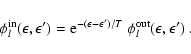 |
(A.13) |
If for a particular
scattering process the energy transfer between neutrinos and
target particles
can be neglected, we have
![]() ,
and
the source terms given by Eqs. (A.10), (A.11),
(A.12)
simplify to
,
and
the source terms given by Eqs. (A.10), (A.11),
(A.12)
simplify to
Applying the procedures outlined in Sect. A.1.2
to the collision integral for the process of thermal emission and
absorption of neutrino-antineutrino pairs by electron positron
pairs and related reactions (e.g., nucleon-nucleon bremsstrahlung), the
corresponding source terms read (see Bruenn 1985; Pons et al. 1998):
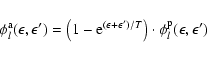 |
(A.21) |
In the following we describe the implementation of the various neutrino-matter interactions into our transport scheme. The expressions are mainly taken from the works of Tubbs & Schramm (1975), Schinder & Shapiro (1982), Bruenn (1985), and Mezzacappa & Bruenn (1993b,c).
All average values of the source terms within individual energy bins
(cf. Eq. (20)) are approximated to zeroth
order by assuming the integrand to be a piecewise constant function of
the neutrino energy ![]() ,
and hence:
,
and hence:
In the standard description of neutrino-nucleon interactions
(see Tubbs & Schramm 1975; Bruenn 1985; Mezzacappa & Bruenn 1993c),
many-body effects for the nucleons in the dense medium, energy
transfer between leptons and nucleons as well as nucleon thermal
motions are ignored.
The corresponding simplifications allow for a straightforward
implementation of the processes, using Eq. (A.5) for the
charged-current reactions and
Eqs. (A.15)-(A.17) for the neutral-current
scatterings, respectively. Expressions for
![]() and the
Legendre coefficients
and the
Legendre coefficients
![]() ,
,
![]() can be
computed from the rates given by Bruenn (1985) and Mezzacappa & Bruenn (1993c).
can be
computed from the rates given by Bruenn (1985) and Mezzacappa & Bruenn (1993c).
For absorption of electron neutrinos by free neutrons
(
![]() )
the final result for the opacity is:
)
the final result for the opacity is:
 |
(A.27) |
Scattering of neutrinos off free nucleons (![]() or
or ![]() )
is mediated by neutral
currents only, which makes the distinction between neutrinos and
antineutrinos unneccessary.
Neglecting nucleon recoil and nucleon thermal motions, the
isoenergetic kernel obeys
)
is mediated by neutral
currents only, which makes the distinction between neutrinos and
antineutrinos unneccessary.
Neglecting nucleon recoil and nucleon thermal motions, the
isoenergetic kernel obeys
![]() (e.g. Bruenn 1985; Mezzacappa & Bruenn 1993c), which implies
(e.g. Bruenn 1985; Mezzacappa & Bruenn 1993c), which implies
![]() .
The non-vanishing Legendre coefficients read
.
The non-vanishing Legendre coefficients read
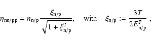 |
(A.31) |
As in the case of charged-current reactions with free nucleons,
neutrino absorption and emission by heavy nuclei
(
![]() )
is implemented
by using Eq. (A.5).
For calculating the opacity of this process
we adopt the description employed by Bruenn (1985) and
Mezzacappa & Bruenn (1993c):
)
is implemented
by using Eq. (A.5).
For calculating the opacity of this process
we adopt the description employed by Bruenn (1985) and
Mezzacappa & Bruenn (1993c):
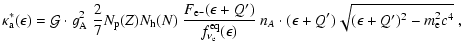 |
(A.32) |
We use reaction rates for coherent neutrino scatterings off nuclei
which include corrections due to the "nuclear form factor''
(following an approximation by Mezzacappa & Bruenn 1993c; Bruenn & Mezzacappa 1997), and
ion-ion correlations (as described in Horowitz 1997).
For a detailed discussion of the numerical handling of both
corrections, see the appendix of Bruenn & Mezzacappa
(1997). The result of the latter reference can readily be
used to calculate
![]() ,
the contribution of coherent
scattering to the rhs of the first order moment equation.
For the Boltzmann equation,
we have to make a minor additional approximation:
The correction factor
,
the contribution of coherent
scattering to the rhs of the first order moment equation.
For the Boltzmann equation,
we have to make a minor additional approximation:
The correction factor
![]() as provided by Horowitz (1997)
applies for the transport opacity and thus for the combination
as provided by Horowitz (1997)
applies for the transport opacity and thus for the combination
![]() (which is given by Bruenn & Mezzacappa 1997) but not
necessarily for the
Legendre coefficients
(which is given by Bruenn & Mezzacappa 1997) but not
necessarily for the
Legendre coefficients ![]() and
and ![]() individually, which are
needed for calculating the collision integral
individually, which are
needed for calculating the collision integral
![]() for
the Boltzmann equation.
We nevertheless assume here that
for
the Boltzmann equation.
We nevertheless assume here that
![]() .
This implies
.
This implies
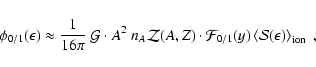 |
(A.33) |
| := |  |
||
| := |  |
(A.34) | |
| y | := |  |
![\begin{displaymath}\mathcal{Z}(A,Z):=
\left[(C_{\rm A}-C_{\rm V})+(2-C_{\rm A}-C_{\rm V})\frac{2Z-A}{A}\right]^2
~\cdot
\end{displaymath}](/articles/aa/full/2002/46/aa2451/img708.gif) |
(A.35) |
For the scattering of neutrinos off charged leptons,
we approximate the dependence of the scattering kernel on the
scattering angle by truncating the Legendre expansions
(Eqs. (A.10)-(A.12)) at
![]() .
For our purposes, this has been shown to provide a sufficiently
accurate approximation (see Smit & Cernohorsky 1996; Mezzacappa & Bruenn 1993b), in
particular also because the total scattering rate is correctly
represented.
Expressions for the Legendre coefficients are taken from the
works of Yueh & Buchler (1977), Mezzacappa & Bruenn (1993b), Cernohorsky (1994), Smit & Cernohorsky (1996):
.
For our purposes, this has been shown to provide a sufficiently
accurate approximation (see Smit & Cernohorsky 1996; Mezzacappa & Bruenn 1993b), in
particular also because the total scattering rate is correctly
represented.
Expressions for the Legendre coefficients are taken from the
works of Yueh & Buchler (1977), Mezzacappa & Bruenn (1993b), Cernohorsky (1994), Smit & Cernohorsky (1996):
Calculating the Legendre coefficients
![]() is a computationally
expensive task, since for all combinations
is a computationally
expensive task, since for all combinations
![]() and all radial grid points numerical integrals
over the energy of the charged leptons (Eq. (A.37)) have to be
carried out.
It is, however, sufficient to explicitly compute
and all radial grid points numerical integrals
over the energy of the charged leptons (Eq. (A.37)) have to be
carried out.
It is, however, sufficient to explicitly compute
![]() for
for
![]() .
The missing coefficients can be obtained by exploiting a number of
symmetry properties (see Cernohorsky 1994).
In doing so, not only the
computational work is reduced by almost a factor of two, but even more
importantly, detailed balance
(
.
The missing coefficients can be obtained by exploiting a number of
symmetry properties (see Cernohorsky 1994).
In doing so, not only the
computational work is reduced by almost a factor of two, but even more
importantly, detailed balance
(
![]() ,
if
,
if
![]() )
can be verified
for the employed approximation and discretization of the
collision integral and its
angular moments to within the roundoff error of the machine, provided
that all integrals over neutrino energies are approximated by simple
zeroth-order quadrature formulae (cf. (Eq. A.22)).
Similarly, one can also verify the conservation of
particle number (Eq. (A.14)) in the corresponding finite
difference representation.
)
can be verified
for the employed approximation and discretization of the
collision integral and its
angular moments to within the roundoff error of the machine, provided
that all integrals over neutrino energies are approximated by simple
zeroth-order quadrature formulae (cf. (Eq. A.22)).
Similarly, one can also verify the conservation of
particle number (Eq. (A.14)) in the corresponding finite
difference representation.
In our neutrino transport code the dependence of the source terms on
the neutrino distribution
and its angular moments is treated fully implicitly in time, i.e. the
time index of the corresponding quantities in
Eqs. (A.10)-(A.12) reads fn+1 and
Ln+1l.
The thermodynamic quantities and the composition of the stellar matter
which are needed to calculate the Legendre coefficients for
inelastic scattering of neutrinos, however, are computed from
![]() and
and
![]() ,
representing the
specific internal energy and electron fraction at the time level after
the hydrodynamic substeps (cf. Sect. 3.6.1).
This allows one to save computer time since the Legendre coefficients
must be computed only once at the beginning of each transport time step.
Comparing to results obtained with a completely time-implicit
implementation of the source terms (i.e. using
,
representing the
specific internal energy and electron fraction at the time level after
the hydrodynamic substeps (cf. Sect. 3.6.1).
This allows one to save computer time since the Legendre coefficients
must be computed only once at the beginning of each transport time step.
Comparing to results obtained with a completely time-implicit
implementation of the source terms (i.e. using
![]() and
and
![]() for determining the stellar conditions that enter the
computation of the Legendre coefficients) we have found no
differences in the solutions during the core-collapse phase, where
neutrino-electron scattering plays an important role in redistributing
neutrinos in energy space and thus couples the neutrino transport to the
evolution of the stellar fluid.
for determining the stellar conditions that enter the
computation of the Legendre coefficients) we have found no
differences in the solutions during the core-collapse phase, where
neutrino-electron scattering plays an important role in redistributing
neutrinos in energy space and thus couples the neutrino transport to the
evolution of the stellar fluid.
Following the suggestion of Pons et al. (1998) we
truncate the Legendre series (A.18)-(A.20) for the
pair-production kernels at
![]() .
The Legendre coefficients are given by (Bruenn 1985; Pons et al. 1998)
.
The Legendre coefficients are given by (Bruenn 1985; Pons et al. 1998)
Legendre coefficients for the nucleon-nucleon bremsstrahlung process,
assuming nonrelativistic nucleons, are
calculated by using the rates given in Hannestad & Raffelt (1998).
The non-vanishing coefficients read:
The production processes of neutrino-antineutrino pairs both by
the annihilation of
![]() pairs and by the
nucleon-nucleon bremsstrahlung are implemented into the discretized
equations (Eqs. (21), (22), (28),
(29)) by applying the techniques described for the
inelastic scattering reactions (see Sect. A.2.4).
pairs and by the
nucleon-nucleon bremsstrahlung are implemented into the discretized
equations (Eqs. (21), (22), (28),
(29)) by applying the techniques described for the
inelastic scattering reactions (see Sect. A.2.4).
![$\displaystyle \frac{\partial}{\partial \mu}
\left[
\left(1-\mu^2\right)\left\{
...
...R}
-\frac{1}{c}{\cal D}_t\Lambda\Big)
-{\cal D}_a\Phi \right\}~{\cal I}
\right]$](/articles/aa/full/2002/46/aa2451/img78.gif)
![$\displaystyle \frac{\partial}{\partial \epsilon}
\left[
\epsilon~\Big(
\left(1-...
...}
+\mu^2\frac{1}{c}{\cal D}_t\Lambda
+\mu {\cal D}_a\Phi
\Big)~{\cal I}
\right]$](/articles/aa/full/2002/46/aa2451/img79.gif)
![$\displaystyle \frac{\partial}{\partial \mu}\left[(1-\mu^2)
\left\{\mu\Big(\frac...
...r}\Big)-\frac{1}{c}\frac{\partial \beta}{\partial t} \right\}~
{\cal I} \right]$](/articles/aa/full/2002/46/aa2451/img96.gif)
![$\displaystyle \frac{\partial}{\partial \epsilon}\left[\epsilon~\Big((1-\mu^2)
\...
...ial
r}+\mu \frac{1}{c}\frac{\partial \beta}{\partial t} \Big)
~{\cal I} \right]$](/articles/aa/full/2002/46/aa2451/img97.gif)
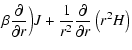
![$\displaystyle \frac{\partial}{\partial \epsilon}\left[\epsilon\left(\frac{\beta...
...eta}{\partial r}K+\frac{1}{c}\frac{\partial \beta}{\partial t}H
\right) \right]$](/articles/aa/full/2002/46/aa2451/img100.gif)
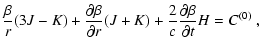
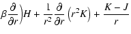
![$\displaystyle \frac{\partial}{\partial
\epsilon}\left[\epsilon~\left(\frac{\bet...
...eta}{\partial r}L+\frac{1}{c}\frac{\partial \beta}{\partial t}K
\right) \right]$](/articles/aa/full/2002/46/aa2451/img103.gif)
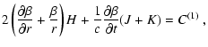

![$\displaystyle \left[\frac{\partial \beta}{\partial r}\right]_{
i+{\frac{1}{2}}}...
...{ i+{\frac{1}{2}},j+{\frac{1}{2}}}\; J_{ i+{\frac{1}{2}},j+{\frac{1}{2}}}^{n+1}$](/articles/aa/full/2002/46/aa2451/img166.gif)
![$\displaystyle \frac{2}{c}\left[\frac{\partial \beta}{\partial t}\right]_{i+{\fr...
...{1}{2}},j+{\frac{1}{2}}}
= {C^{(0)}}^{n+1}_{i+{\frac{1}{2}},j+{\frac{1}{2}}}
~,$](/articles/aa/full/2002/46/aa2451/img167.gif)

![$\displaystyle \left[\frac{\partial \beta}{\partial r}\right]_{i}\;H_{ i,j+{\fra...
...{f_K})\; J^{n+1}]}_{ i,j+{\frac{1}{2}}}
={C^{(1)}}^{n+1}_{i,j+{\frac{1}{2}}}
~.$](/articles/aa/full/2002/46/aa2451/img173.gif)
![$\displaystyle u_{i+{\frac{1}{2}},j}:=
\left[\frac{\beta}{r}\right]_{i+{\frac{1}...
...rtial \beta}{\partial t}\right]_{i+{\frac{1}{2}}}
{[f_H]}_{i+{\frac{1}{2}},j}~,$](/articles/aa/full/2002/46/aa2451/img177.gif)
![$\displaystyle w_{i,j}:=
\left[\frac{\beta}{r}\right]_{i}{[f_H-f_L]}_{i,j}
+ \le...
... \frac{1}{c}\left[\frac{\partial \beta}{\partial t}\right]_{i}
{[f_K]}_{i,j}
~.$](/articles/aa/full/2002/46/aa2451/img178.gif)
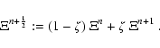
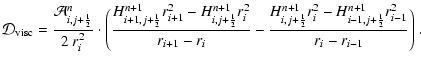
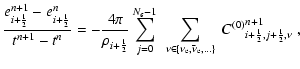
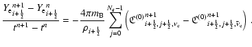


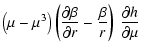
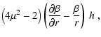
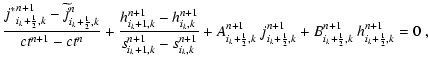
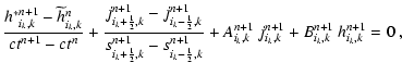
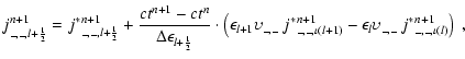
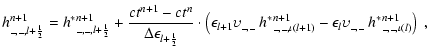
![\begin{displaymath}
\iota(l):=
\left\{
\begin{array}{ll}
l-\frac{1}{2} &{\rm for...
...~, \\ [2mm]
l+\frac{1}{2} &{\rm else}~, \\
\end{array}\right.
\end{displaymath}](/articles/aa/full/2002/46/aa2451/img260.gif)
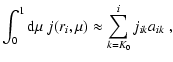
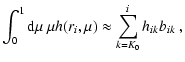
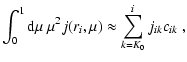
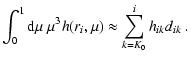
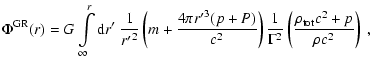
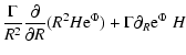
![$\displaystyle \frac{\partial}{\partial \epsilon}\left[
\epsilon~\Big(
{\rm e}^{...
...+c^{-1} {\rm D}_t \Lambda~ K
+\Gamma
\partial_R {\rm e}^{\Phi}~ H
\Big) \right]$](/articles/aa/full/2002/46/aa2451/img332.gif)
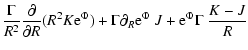
![$\displaystyle \frac{\partial}{\partial \epsilon}\left[
\epsilon~\Big(
{\rm e}^{...
...+c^{-1} {\rm D}_t \Lambda~ L
+\Gamma
\partial_R {\rm e}^{\Phi}~ K \Big)
\right]$](/articles/aa/full/2002/46/aa2451/img336.gif)

![$\displaystyle \frac{\partial}{\partial \epsilon}\left[
\epsilon~\Big(
{\rm e}^{...
...D}_t \Lambda~ {\cal K}
+\Gamma\partial_R {\rm e}^{\Phi}~ {\cal H}
\Big) \right]$](/articles/aa/full/2002/46/aa2451/img340.gif)
![$\displaystyle \frac{\partial}{\partial \epsilon}\left[
\epsilon~\Big(
{\rm e}^{...
...}_t \Lambda~ {\cal L}
+\Gamma
\partial_R {\rm e}^{\Phi}~ {\cal K} \Big)
\right]$](/articles/aa/full/2002/46/aa2451/img344.gif)
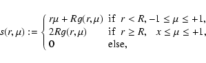
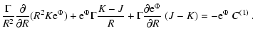
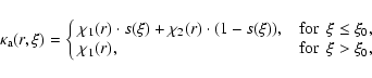
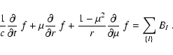
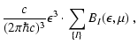
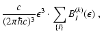

![\begin{displaymath}
B_{\rm AE}(\epsilon,\mu)=
\kappa_{\rm a}^*(\epsilon)[f^{\rm eq}(\epsilon)-f(\epsilon,\mu)]
~.
\end{displaymath}](/articles/aa/full/2002/46/aa2451/img588.gif)
![$\displaystyle B_{\rm S}(\vec{q})=
\int
\frac{{\rm d}^3\vec{\vec{q'}}~}{(2\pi)^3...
...},\vec{q'})
-f_\nu(1-f'_\nu)\widetilde{R}^{\rm out}(\vec{q},\vec{q'})\right]
~,$](/articles/aa/full/2002/46/aa2451/img592.gif)
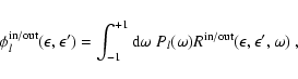

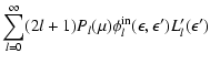
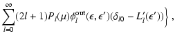

![$\displaystyle B^{(1)}_{\rm S}(\epsilon) =
2\pi~\int_0^\infty {\rm d}\epsilon'~ ...
...on)]
\phi_l^{\rm out}(\epsilon,\epsilon')(\delta_{l0}-L'_l(\epsilon'))\Big\}
~,$](/articles/aa/full/2002/46/aa2451/img627.gif)
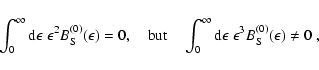
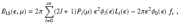

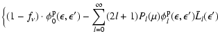
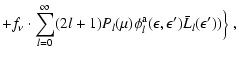
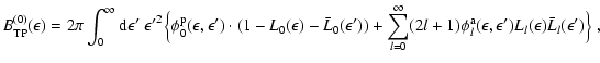
![$\displaystyle B^{(1)}_{\rm TP}(\epsilon) =
2\pi\int_0^\infty {\rm d}\epsilon'~ ...
...n')
[
(l+1)L_{l+1}(\epsilon)+l L_{l-1}(\epsilon)
]\bar{L}_l(\epsilon')
\Big\}~.$](/articles/aa/full/2002/46/aa2451/img642.gif)
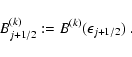

![$\displaystyle 2\int\frac{{\rm d}^3\vec{p}~}{(2\pi\hbar
c)^3}F_{\rm n}(\epsilon)[1-F_{\rm p}(\epsilon)]$](/articles/aa/full/2002/46/aa2451/img665.gif)
![$\displaystyle \frac{n_{\rm p}-n_{\rm n}}{\exp{\left[\psi_{\rm p}-\psi_{\rm n}\right]}-1}
~,$](/articles/aa/full/2002/46/aa2451/img666.gif)
![$\displaystyle \frac{{\cal G}}{8\pi}\cdot
\left\{
\begin{array}{ll}
\eta_{\rm nn...
..._{\rm V}-1)^2+\frac{3}{4}g_{\rm A}^2\right] &({\rm for\ p})~,\end{array}\right.$](/articles/aa/full/2002/46/aa2451/img677.gif)
![$\displaystyle \frac{{\cal G}}{24\pi}\cdot
\left\{
\begin{array}{ll}
\eta_{\rm n...
..._{\rm V}-1)^2-\frac{1}{4}g_{\rm A}^2\right]
&({\rm for\ p})~.\end{array}\right.$](/articles/aa/full/2002/46/aa2451/img679.gif)