2 Model description

Figure 1: The heliospheric interface is the region of the solar wind interaction with LIC. The heliopause is a contact discontinuity, which separates the plasma wind from interstellar plasmas. The termination shock decelerates the supersonic solar wind. The bow shock may also exist in the interstellar medium. The heliospheric interface can be divided into four regions with significantly different plasma properties: 1) supersonic solar wind; 2) subsonic solar wind in the region between the heliopause and termination shock; 3) disturbed interstellar plasma region (or "pile-up'' region) around the heliopause; 4) undisturbed interstellar medium.

2.1 Hydrogen distributions

The interaction of the solar wind with the interstellar medium influences the distribution of interstellar atoms inside the heliosphere. At the present time, there is no doubt that the Local Interstellar Cloud is partly ionized. The plasma component of the LIC interacts with the solar wind plasma and forms the heliospheric interface (Fig. 1). Interstellar H atoms interact with the plasma component by charge exchange. This interaction strongly influences both plasma and neutral components. The main difficulty in the modeling of the H atom flow in the heliospheric interface is its kinetic character due to the large, i.e. comparable to the size of the interface, mean free path of H atoms with respect to the charge exchange process. In this paper, to get the H atom distribution in the heliosphere and heliospheric interface structure we use the self-consistent model developed by Baranov & Malama (1993). The kinetic equation for the neutral component and the hydrodynamic Euler equations were solved self-consistently by the method of global interactions. To solve the kinetic equation for H atoms, an advanced Monte Carlo method with splitting of trajectories (Malama 1991) was used. Basic results of the model were reported by Baranov & Malama (1995), Izmodenov et al. (1999), Izmodenov (2000), Izmodenov et al. (2001).

Figure 2: Number densities and velocities of four populations of H atoms as functions of heliocentric distance in the upwind direction. 1 designates atoms created in the supersonic solar wind, 2 atoms created in the heliosheath (SSWAs), 3 atoms created in the disturbed interstellar plasma (HIAs), and 4 original (or primary) interstellar atoms (PIAs). Number densities are normalized to $n_{\rm H,LIC}$, velocities are normalized to $V_{\rm LIC}$. It is assumed that $n_{\rm H,LIC}=0.2$ cm-3, $n_{\rm p,LIC}=0.04$ cm-3.

Hydrogen atoms newly created by charge exchange have the velocities of their ion partners in charge exchange collisions. Therefore, the parameters of these new atoms depend on the local plasma properties. It is convenient to distinguish four different populations of atoms depending on where in the heliospheric interface they originated. Population 1 corresponds to the atoms created in the supersonic solar wind. It is denoted SSWA (supersonic solar wind atoms). Population 2 (denoted HSWA, hot solar wind atoms) represents the atoms originating in the heliosheath. Population 3 (HIA, hot interstellar atoms) are the atoms created in the disturbed interstellar wind. We will call original (or primary) interstellar atoms population 4 (PIA, primary interstellar atoms). The number densities and mean velocities of these populations are shown in Fig. 2 as functions of the heliocentric distance. The main results of the model for the H atom populations can be summarized as follows:

PIAs are significantly filtered (i.e. their number density is reduced) before reaching the termination shock. Since slow atoms have a smaller mean free path compared to fast atoms, they undergo more charge exchange. This kinetic effect, called selection, results in a deviation of the interstellar distribution function from Maxwellian (Izmodenov et al. 2001). The selection also results in $\sim$10% increase of the primary atom mean velocity at the termination shock (Fig. 2C).

HIAs are created in the disturbed interstellar medium by charge exchange of primary interstellar neutrals and protons decelerated by the bow shock. The secondary interstellar atoms collectively make up the H wall, a density increase at the heliopause. The H wall has been predicted by Baranov et al. (1991) and detected toward $\alpha$ Cen (Linsky & Wood 1996). At the termination shock, the number density of the secondary neutrals is comparable to the number density of the primary interstellar atoms (Fig. 2A, dashed curve). The relative abundances of PIAs and HIAs entering the heliosphere depends on the degree of ionization in the interstellar medium. It has been shown by Izmodenov et al. (1999) that the relative abundance of HIAs inside the termination shock increases with increasing interstellar proton number density. The bulk velocity of HIAs is about 18-19 km s^-1. This population approaches the Sun. The velocity distribution of HIAs is not Maxwellian. The velocity distributions of different populations of H atoms were calculated in Izmodenov et al. (2001) for different directions from upwind. The fine structures of the velocity distribution of the primary and secondary interstellar populations vary with direction. These variations of the velocity distributions reflect the geometrical pattern of the heliospheric interface. The velocity distributions of the interstellar atoms can provide a good diagnostic of the global structure of the heliospheric interface.

The third component of the heliospheric neutrals, HSWAs, corresponds to the neutrals created in the heliosheath from hot and compressed solar wind protons. The number density of this population is an order of magnitude smaller than the number densities of the primary and secondary interstellar atoms. This population has a minor importance for interpretations of Ly $\alpha$ and pickup ion measurements inside the heliosphere. However, some of these atoms may probably be detected by Ly$\alpha$ hydrogen cell experiments due to their large Doppler shifts. Due to their high energies, the particles influence the plasma distributions in the LIC. Inside the termination shock the atoms propagate freely. Thus, these atoms can be a source of information on the plasma properties in the place of their birth, i.e. the heliosheath.

The last population of heliospheric atoms is SSWAs, the atoms created in the supersonic solar wind. The number density of this atom population has a maximum at $\sim$5 AU from the sun. At this distance, the number density of population 1 is about two orders of magnitude smaller that the number density of the interstellar atoms. Outside the termination shock the density decreases faster than 1/r²where r is the heliocentric distance (curve 1, Fig. 2B). The mean velocity of population 1 is about 450 km s^-1, which corresponds to the bulk velocity of the supersonic solar wind. The supersonic atom population results in the plasma heating and deceleration upstream of the bow shock. This leads to the decrease of the Mach number ahead of the bow shock.

SSWAs velocities are Doppler shifted out of the solar H Lyman $\alpha$ line and therefore are not detectable in by interplanetary Lyman $\alpha$ measurements. Atoms of the three other populations penetrate the heliosphere and may backscatter solar Ly$\alpha$ photons. This is in contrast to the classical hot model (Thomas 1978; Lallement et al. 1985) which assumed that at large heliocentric distance the velocity distribution is Maxwellian and unperturbed by the heliospheric interface interaction.

Table 1 gives a summary of the different H populations in the heliosphere. The number of the region of origin of each population, as shown in Fig. 1, is also given in the table. We also give the range of variation of the number density of the population in the inner heliosphere as shown in Fig. 2.

 

Table 1: H populations summary.

Acronym	Full name	scatter H Ly-a	Origin	Nh/Nlic Range
SSWA	Supersonic Solar Wind Atoms	No	Region 1	10-3-10-2
HSWA	Hot Solar Wind Atoms	Yes	Region 2	10-3-10-1
HIA	Hot Interstellar Atoms	Yes	Region 3	0.1-0.3
PIA	Primary Interstellar Atoms	Yes	Region 4	0.1-0.3

In what follows, we will include the full distribution of the three populations (2, 3 and 4 from Table 1) that can actually backscatter solar Lyman $\alpha$ photons to compute the interplanetary UV background. Each population will be referred to by use of its label (PIA, HIA, HSWA). The hydrogen distribution model will be called three population model, denoted 3p model, because the SSWA is invisible to Ly$\alpha$ light.

For reference, the parameters of the hydrogen distribution model are given by

LIC parameters
Proton number density	0.04 cm-3
Hydrogen number density	0.2 cm-3
Bulk velocity	25 km s-1
Temperature	5700 K
Solar parameters
Radiation pressure to gravitation ($\mu$)	0.75
Proton number density at Earth	7 cm-3
Solar wind velocity	450 km s-1

2.2 Multi-component radiative transfer calculations

2.2.1 Radiative transfer model assumptions

In this study we use the results of two radiative transfer models following the scheme described by Quémerais (2000). Our method combines a standard iterative computation of the first-order and second-order scattering terms with Monte Carlo simulations used to compute the higher orders of scattering (i.e., photons that are scattered more than two times). The second-order scattering term is computed by integration over the whole sky of the first-order component. It is also computed independently by the Monte Carlo simulation. This provides a way to check the validity of both methods (Quémerais 2000).

The iterative scheme, i.e. computing order $n_{\rm s}$ from integration over the whole sky of terms of scattering order $n_{\rm s} - 1$, could theoretically be applied to any order (see Sect. 2.3 of Quémerais 2000). However, starting from $n_{\rm s} = 3$, it is much more efficient to use a Monte Carlo approach.

The general assumptions of our model are the following:

• The photon source frequency profile is derived from the SUMER/SOHO measurements (Lemaire et al. 1998). The source profile is shown in Quémerais (2000).

• The density distribution of the three populations is symmetrical around the wind axis going through sun center.

• The local distribution of hydrogen atoms is represented by the sum of three components.

• In each point of the heliosphere, the local distribution of each component is described by 6 values: a number density, a mean velocity and three temperatures which are the temperatures of the velocity distribution projected on the three directions of the local frame. These three temperatures can be different, which means that the local distribution is not necessarily a Maxwell-Boltzman distribution.

• The scattering process is computed following the Angle Dependent Partial Frequency Redistribution (Mihalas 1970). This means that the frequency of the outgoing photons depends on the frequency of the incoming photons, the scattering angle and the velocity distribution at the point of scattering. The numerical expressions of the redistribution function is given in Quémerais (2000).

• The scattering redistribution function includes the phase function given by Brandt & Chamberlain (1959). The improved phase function by Brasken & Kyrölä (1998) has not been included here because it leads to changes which are much lower than the expected accuracy of our Monte Carlo computation.

The Monte Carlo model has the following boundary conditions

• The solar photons are randomly generated following the solar H Lyman $\alpha$ line profile of Lemaire et al. (1998). The source is spatially isotropic.

• For each scattering, the new frequency of the photon is randomly generated using the ADPFR redistribution function and the local hydrogen distribution parameters at the point of scattering.

• There is no limit for the number of scatterings.

• The model stops following a photon once it has reached a distance of 600 AU from the Sun. This limit was obtained by comparison of different MC runs. It was shown that increasing this distance has no effect on the emissivity within 100 AU from the Sun.

Previous works have used the assumption of Complete Frequency Redistribution (Keller et al. 1981; Hall 1992; Quémerais & Bertaux 1993), for which the frequency of the outgoing photon only depends on the local density distribution at the point of scattering. Unfortunately, this simpler assumption does not allow for an exact computation of backscattered line profiles because it neglects of the incoming photon frequency profile. This applies to a medium with large optical thickness where many scatterings occur, not in the inner heliosphere. To be able to compute exact line profiles, we had to implement a scheme based on the actual Angle Dependent Partial Redistribution Function described by Mihalas (1970). Quémerais (2000) has devoted a whole section (Sect. 4) to the comparison between CFR and ADPFR results.

2.2.2 Terminology

This section tries to clarify the different terms used in what follows.

The physical quantities that can be measured are intensities. They correspond to a number of photons collected per surface unit per time unit per solid angle unit. Intensities are not local, they are integrated over a line of sight. Locally, the emissivity measures the number of photons emitted in all directions per volume unit per time unit. It can be divided into its spatial (per solid angle unit) and spectral (per frequency unit) components.

The only exact way to compute the interplanetary H Lyman $\alpha$background requires a full computation of the multiple scattering process using an angle dependent partial frequency redistribution function. This must be coupled to a complete distribution of the density, velocity and temperature of the H atoms in the heliosphere. However, due to the complexity of the task, various approximations have been developed to speed up the computation.

Figure 3: Illustration of the scattering process of a Lyman alpha photon on a H atom in the heliosphere and its observation by an instrument in the heliosphere. The single scattering case is shown by the path L1 and L2. The multiple scattering case can be represented by M1, M2 and L2 but may involve more scatterings. The diamonds are used to show that the density increases with solar distance. This means that the thin medium of the inner heliosphere is surrounded by a denser medium which contributes to the intensity seen at 1 AU.

In Fig. 3, we present a simple observing scenario. The intensity observed for a given Line Of Sight (LOS) is the integral over the line of sight of the local emissivity (Eq. (15) in Quémerais 2000). This emissivity is split in two terms. The primary term refers to photon which are scattered only once between the source and the observer (path L1+L2 in Fig. 3). The secondary term refers to photons that are scattered more than once (e.g. path M1+M2+L2 in Fig. 3). Many approximations neglect the secondary term. We will come back to that point later.

Approximations that neglect the secondary term:

• The first one is the optically thin approximation (noted OT). This corresponds to the assumption that extinction can be neglected and as a consequence that photons are scattered only once in the heliosphere. This assumption often gives correct intensity estimates in the inner heliosphere because extinction and multiple scattering tend to compensate one another (Keller et al. 1981; Hall 1992; Quémerais & Bertaux 1993). Its results tend to underestimate the line width in the case of the hot model (Quémerais 2000).

• The second type of computation is often referred to as the primary intensity (noted Primary here). It computes exactly the intensity due to single scattering, i.e. extinction is applied between the source and the observer. In the inner heliosphere, the primary term, noted I₀, represents roughly 60% of the intensity seen from 1 AU (Quémerais 2000). This may seem surprising since it is easy to remark that at one AU from the sun, the interplanetary medium is optically thin at Lyman $\alpha$. However, we must not forget that the intensity is integrated over a large distance on the line of sight and that a significant fraction of the total intensity comes from outside the inner heliosphere where the medium is optically thicker.

• A third type of computation was used by Bertaux et al. (1985) to improve the accuracy of the optically thin case without going into the details of an actual radiative transfer computation. Is is often referred to as the self-absorbed computation (noted SA). It is identical to the optically thin calculation except that extinction on the line of sight between the scattering point and the observer is included. It is then an intermediate scheme between the optically thin case and the primary term which also includes extinction between the source and the scattering point.

Those three types of approximations can be used either with the CFR or the ADPFR redistribution function. Table 2 sums up the different hypotheses.

 

 

Table 2: Model approximation summary.

Approximation		noted	Extinction		Secondary term
			on L1	on L2	included
Optically Thin	(OT)	$I_{\rm ot}$	No	No	No
Primary Term	(Primary)	I0	Yes	Yes	No
Self-Absorbed	(SA)	$I_{\rm sa}$	No	Yes	No

Following Quémerais (2000), we note that none of these numerical schemes fully represents the actual physical processes and that it is necessary to include all scattering orders to have a correct representation of the interplanetary Lyman $\alpha$ background. Numerical estimates of the errors introduced by these approximations are given in Quémerais (2000).

We will also repeat the remarks of Sect. 3 of Quémerais (2000). Scherer & Fahr (1996) and subsequent works claim that the secondary intensity term is negligible and that the primary term is enough to compute exactly the UV background in the inner heliosphere. We found that this is inexact here as already stated in Quémerais (2000).

It is clear that the interplanetary medium is optically thin at 1 AU. However, optical thickness increases with solar distance. At 10 AU, it is not optically thin anymore. Photons that cross the inner heliosphere are scattered at greater distance from the sun and a fraction of these contributes to the intensity seen at one AU. This is illustrated in Fig. 3.

More recently, Scherer & Scherer (2001) have considered the ratio of the backscattered intensity by He atoms at 58.4 nm with the resonance scattering of H atoms (121.6 nm) measured by the same instrument on Pioneer 10. They found that the ratio of both UV glow data is fairly constant over roughly 30 AU, between 1972 to 1984. From this remark and using the fact that the interplanetary medium is optically thin at 58.4 nm, they conclude that the H Lyman $\alpha$ UV glow can be modeled by an optically thin approximation "because otherwise the ratio would not be constant for such a large heliocentric distance" (quote from Scherer & Scherer 2001, pages 137-138).

This last sentence is inexact. One of the most striking results of the various models of Keller et al. (1981), Hall (1992), Quémerais & Bertaux (1993) is that the intensity ratio of an optically thin model with a full radiative transfer model is roughly constant over a range of distances to the sun. The actual range of distance over which the ratio is more or less constant depends on the density model used in the model. This is due to a cancellation of effects between extinction and multiple scattering terms. A similar result is obtained by Quémerais (2000) (Fig. 8 of that paper) in the case of ADPFR. However, the value of the ratio is not the same if one considers observations in the upwind direction or the downwind direction. It is well known that the upwind to downwind intensity ratio is not correctly modeled by an optically thin approxmation (Keller et al. 1981; Quémerais 2000).

2.3 Model accuracy

In this section, we present estimates of the model accuracy and numerical stability. First we consider the radiative transfer Monte Carlo code. Second, we discuss error propagation between the Monte Carlo computation of hydrogen atom distributions and the Monte Carlo code used to compute the multiple scattering terms.

2.3.1 Radiative transfer Monte Carlo model

For the Monte Carlo model of multiple scattering, we simulate the path of a large number of photons emitted by the sun (Quémerais 2000). The local emissivity is obtained by keeping track of where the simulated photons are scattered and storing this information in a set of counters defined on a spatial and spectral grid. This means that at the end of the run, each grid point has counted a number of scatterings. The corresponding 1-$\sigma$ statistical error for each counter is equal to the square root of the number of counts.

From this, we have derived the statistical error for each of the physical quantities used by applying the law of propagation of errors. This is expressed by

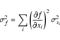$$\sigma_f^2 = \sum_i \left( \frac{\partial f}{\partial x_i} \right)^2 \sigma_{x_i}^2$$ (1)

where the quantity f is a function of the independent variables x_i. $\sigma_{x_i}$ expresses the individual statistical errors of the variables, $\sigma_f$ is the statistical error of the derived quantity, i.e. emissivity or intensity in our case.

The model used in this work computed 160 million photon trajectories. The corresponding statistical accuracy is very good. The 1-$\sigma$ statistical error for total intensities (i.e. integrated over spectral range) is everywhere lower than 5 Rayleighs. The corresponding model accuracies for total intensities vary between 1% to 5% according to the line of sight. In Fig.  6, we show the individual errors in each spectral bin.

The 1-$\sigma$ statistical error for apparent line doppler shifts is smaller than 0.5 km s^-1. In most of the cases it is lower than than 0.2 km s^-1 except for lines of sight close to the wind axis where the effective counter size is smaller.

Finally, apparent line temperatures have a 1-$\sigma$ statistical error smaller than 1000 K everywhere. For most of the lines of sight, the error is smaller than 500 K except close to the axis of symmetry of the density model where it reaches 1000 K. Statistical errors for the temperature are shown in Fig. 9.

2.3.2 Error propagation between Monte Carlo models

The last question that arises from our model is the problem of numerical stability. The H atom density and velocity distribution is the result of a Monte Carlo computation (Izmodenov et al. 2001). As stated by these authors, the number density values have an accuracy better than 5%. From this we can deduce the accuracy of model intensities. It is clear that for the optically thin case, multiplying all densities by a factor k, changes the intensities by the same factor. The primary term is simply the optically thin case with extinction on the photon path. This means that all primary terms have a statistical accuracy of 5%.

However, we must also consider the effect of density inaccuracy in our computations of the secondary term due to multiple scattering. If the model is not numerically stable, a small change in density will yield a large change in multiply scattered intensity.

To test this, we ran three new MC models. The original model is noted MC0. A second model, noted MC1, is the same as the previous one except all densities have been multiplied by a factor 1.05. Similarly, MC2 is the same as MC0 except all densities are multiplied by a factor 0.95. Finally, a third attempt (MC3), is the same model as MC0, except densities are multiplied by random numbers between 0.95 and 1.05.

We then compared all secondary emissivities from the various models. It was found that the difference in secondary emissivities between MC1 or MC2 and MC0 is always smaller than  10% within 100 AU of the Sun. The difference of the secondary emissivity between MC2 and MC0 is much smaller, less than 2%. This proves that the model is numerically stable and that a small relative variation in density gives only a small variation in emissivity terms.

Finally, after integration over the line of sight, we found that the difference in secondary intensity between the different models is always less than 20 Rayleighs at 1 AU. This value corresponds to a rough estimate of the upper limit of the statistical error due to the combination of both Monte Carlo codes.