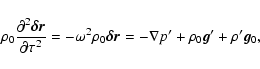
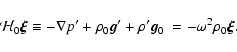
Our aim is to investigate smaller effects like slow streaming large-scale poloidal fields. The first step is to solve the forward problem, i.e., to calculate theoretically the influence on the solar acoustic modes. We will follow the work of Lavely & Ritzwoller (1992). The starting point for these calculations is a reference model; we base our work on "Model S'' from Christensen-Dalsgaard et al. (1996). The reference model describes the Sun as a star in hydrostatic equilibrium. It is one-dimensional, i.e., all physical quantities depend on one variable, the distance r from the solar center. It follows that the solar model is spherically symmetric, non-rotating, non-magnetic, and static.
This reference model is subject to acoustic modes, which are
characteristic spatial displacement patterns
![]() ,
that oscillate with fixed frequencies (
,
that oscillate with fixed frequencies (![]() and
and
![]() are the colatitude and the longitude;
are the colatitude and the longitude; ![]() is the time).
The equation of motion of such an oscillatory displacement
is the time).
The equation of motion of such an oscillatory displacement
![]() with amplitude
with amplitude
![]() and angular frequency
and angular frequency ![]() is derived in
Christensen-Dalsgaard (1998) and is given by
is derived in
Christensen-Dalsgaard (1998) and is given by
Equation (1) has a spectrum of eigensolutions with eigenvalues
![]() ,
where k=(n,l,m) stands for a triplet of indices,
respectively, the radial order, the harmonic degree, and the azimuthal
order. We will concentrate on the p-modes whose restoring force is the
pressure gradient.
,
where k=(n,l,m) stands for a triplet of indices,
respectively, the radial order, the harmonic degree, and the azimuthal
order. We will concentrate on the p-modes whose restoring force is the
pressure gradient.
For a spherical symmetric solar model the solar p-modes are degenerate,
i.e., each p-mode of a multiplet that consists of the 2l+1
eigenfunctions with identical n and l values
has the same frequency
![]() independent of m.
In Fig. 1 we show the spectrum or
independent of m.
In Fig. 1 we show the spectrum or ![]() diagram of the
p-modes with
diagram of the
p-modes with ![]() and
and
![]() mHz that were
calculated on the basis of "Model S'' (Christensen-Dalsgaard et al. 1996).
mHz that were
calculated on the basis of "Model S'' (Christensen-Dalsgaard et al. 1996).
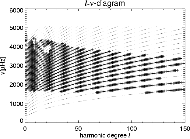 |
Figure 1:
|
In this paper we investigate velocity fields ![]() in the
convection zone; they lift the degeneracy
by an additional advection term in the equation of
motion (1), (Christensen-Dalsgaard 1998; Lavely & Ritzwoller 1992)
in the
convection zone; they lift the degeneracy
by an additional advection term in the equation of
motion (1), (Christensen-Dalsgaard 1998; Lavely & Ritzwoller 1992)
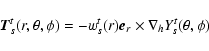
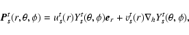
For our purposes ![]() is decomposed into a toroidal and a poloidal
field and the two components are expanded in spherical harmonics
Yst defined by
is decomposed into a toroidal and a poloidal
field and the two components are expanded in spherical harmonics
Yst defined by
![$\displaystyle Y_s^t(\theta,\phi)= \frac{(-1)^{s+t}}{2^s s!}
\left[\frac{(2s+1)(...
...al}{\partial(\cos\theta)}\right]^{s+t}(\sin\theta)^{2s}
{\rm e}^{{\rm i}t \phi}$](/articles/aa/full/2002/46/aa2060/img34.gif) |
(6) |
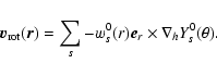
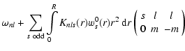
The differential rotation, which is a pure toroidal velocity field,
can be expanded in zonal components of spherical harmonics Ys0
according to Eqs. (7) and (8)
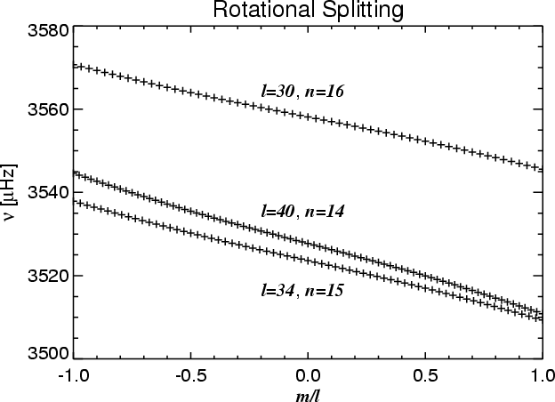 |
Figure 2:
Lifting of degeneracy by differential rotation (solar
|
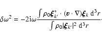
In this section we study the effect of large-scale flows, located in the convection zone, on solar oscillations. By large-scale flows we mean flows that have only poloidal and non-zonal toroidal components. We refer to zonal toroidal components as differential rotation, for which we already did the calculations in the last section.
We focus only on the effect of the poloidal components on the solar
oscillations, because the effect of the non-zonal toroidal flow
components should be the smallest (Roth 2001).
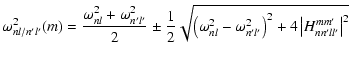
A poloidal flow field will result in a frequency shift of
![]() in the case
(n',l',m')=(n,l,m), because of three
selection rules (Lavely & Ritzwoller 1992). The first two rules arise from
properties of the Wigner 3j symbols which vanish except when
the harmonic degrees l, l', and s satisfy a triangular condition
(Edmonds 1960), i.e.
in the case
(n',l',m')=(n,l,m), because of three
selection rules (Lavely & Ritzwoller 1992). The first two rules arise from
properties of the Wigner 3j symbols which vanish except when
the harmonic degrees l, l', and s satisfy a triangular condition
(Edmonds 1960), i.e.
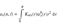
For the numerical determination of the shifted frequencies it is helpful
to limit the number of possible coupling partners by the requirement
![]() with given
with given
![]() .
In principle, we have to include all possible
coupling partners. But according to Eq. (16), the strength of
the coupling decreases with increasing difference in frequency, as can
be seen by an expansion of the square root. This is
characteristic for perturbation theory of quasi-degenerate eigenstates;
it is for this reason that only modes with frequencies in close
vicinity need to be taken into account. For the highest amplitudes of
the velocity fields used in our calculations the contributions become
more and more negligible for frequency differences above
.
In principle, we have to include all possible
coupling partners. But according to Eq. (16), the strength of
the coupling decreases with increasing difference in frequency, as can
be seen by an expansion of the square root. This is
characteristic for perturbation theory of quasi-degenerate eigenstates;
it is for this reason that only modes with frequencies in close
vicinity need to be taken into account. For the highest amplitudes of
the velocity fields used in our calculations the contributions become
more and more negligible for frequency differences above
![]()
![]() Hz. We can thus limit the number of
possible partners and speed up the numerical calculations by setting
Hz. We can thus limit the number of
possible partners and speed up the numerical calculations by setting
![]() without loss of
generality. Moreover the selection rules will further reduce
the number of couplers.
without loss of
generality. Moreover the selection rules will further reduce
the number of couplers.
Coupling of modes leads to additional, and in the case
![]() to asymmetric, shifts in a multiplet, cf. the examples in
Figs. 3 and 4.
to asymmetric, shifts in a multiplet, cf. the examples in
Figs. 3 and 4.
![\begin{figure}
\par\resizebox{8.8cm}{!}{\includegraphics[width=8cm]{ms2060f4.eps}}\end{figure}](/articles/aa/full/2002/46/aa2060/img63.gif) |
Figure 4:
The multiplet l=34, n=15 and its coupling partners affected
by a zonal poloidal flow s=8, t=0,
|
At this point we add a few remarks about the symmetry of the Wigner 3j
symbols and the resulting sensitivity to various flows. These remarks
will become essential for the understanding of the results presented in
Sect. 4. The differential rotation leads to splittings that
are anti-symmetric with respect to m=0 (cf. Fig. 2); the
Wigner 3j symbols that represent these splitting are the
(s l l/0 m -m)-symbols. Due to the third selection rule
the contribution to the frequency shift is non-zero only for odd
s. Therefore the expansion of the rotational splitting was given by
the odd as-coefficients. Conversely the meridional flows lead to
splittings symmetric about m=0 (cf. Fig. 4); the
corresponding Wigner 3j symbols are the
(s l l'/0 m -m)-symbols. Due to the selection rules the
contribution to the frequency shift is non-zero for even
s+l+l'. Therefore the expansion of the meridional-flow-splitting in
terms of functions that are symmetric and anti-symmetric with respect to
m=0 will be given by the expansion coefficients corresponding to the
even functions. Any other poloidal flow field with ![]() will
result in a distribution of the frequency shifts with no symmetry with
respect to m=0, due to the second selection rule (15);
therefore these shifts cannot be assigned to only even or only odd
functions in an expansion.
will
result in a distribution of the frequency shifts with no symmetry with
respect to m=0, due to the second selection rule (15);
therefore these shifts cannot be assigned to only even or only odd
functions in an expansion.
As result of the combined effect of differential rotation and poloidal
velocity fields, the frequencies within a multiplet might be
distributed as shown in the example of Fig. 5 for differential
rotation plus a poloidal velocity field with s=t=8.
![\begin{figure}
\par\resizebox{8.8cm}{!}{\includegraphics[width=8cm]{ms2060f5.eps}}\end{figure}](/articles/aa/full/2002/46/aa2060/img64.gif) |
Figure 5:
Poloidal velocity fields (here s=t=8) lead to a deviation
(+-symbols) from the rotational splitting (dots). To emphasize the
deviation an amplitude
|
Copyright ESO 2002
![\begin{displaymath}\vec{v}(\vec{r})=\sum_{s=0}^{\infty}\sum_{t=-s}^s
\left[\vec{T}_s^t(r,\theta,\phi) + \vec{P}_s^t(r,\theta,\phi)\right] ,
\end{displaymath}](/articles/aa/full/2002/46/aa2060/img35.gif)
![\begin{figure}
\par\resizebox{8cm}{!}{\includegraphics[width=8cm]{ms2060f3.eps}}\end{figure}](/articles/aa/full/2002/46/aa2060/img62.gif)