A&A 395, 99-115 (2002)
DOI: 10.1051/0004-6361:20021153

Numerical simulations of surface convection in a late M-dwarf

H.-G. Ludwig^1,2 - F. Allard² - P. H. Hauschildt^3,2

1 - Lund Observatory, Box 43, 22100 Lund, Sweden
2 - C.R.A.L., École Normale Supérieure, 69365 Lyon Cedex 7, France
3 - Dept. of Physics and Astronomy & Center for Simulational Physics, University of Georgia,
Athens, GA 30602-2451, Greece

Received 17 January 2002 / Accepted 1 August 2002

Abstract
Based on detailed 2D and 3D numerical radiation-hydrodynamics (RHD) simulations of time-dependent compressible convection, we have studied the dynamics and thermal structure of the convective surface layers of a prototypical late-type M-dwarf ( $\ensuremath{T_{{\rm eff}}}\approx 2800\mbox{\rm ~K}$, $\ensuremath{\log g} =5.0$, solar chemical composition). The RHD models predict stellar granulation qualitatively similar to the familiar solar pattern. Quantitatively, the granular cells show a convective turn-over time scale of $\approx$ $100\mbox{\rm ~s}$, and a horizontal scale of $80\mbox{\rm ~km}$; the relative intensity contrast of the granular pattern amounts to 1.1%, and root-mean-square vertical velocities reach 240 m s^-1 at maximum. Deviations from radiative equilibrium in the higher, formally convectively stable atmospheric layers are found to be insignificant allowing a reliable modeling of the atmosphere with 1D standard model atmospheres. A mixing-length parameter of  = 2.1 provides the best representation of the average thermal structure of the RHD model atmosphere while alternative values are found when fitting the asymptotic entropy encountered in deeper layers of the stellar envelope (  = 1.5), or when matching the vertical velocity (  = 3.5). The close correspondence between RHD and standard model atmospheres implies that presently existing discrepancies between observed and predicted stellar colors in the M-dwarf regime cannot be traced back to an inadequate treatment of convection in the 1D standard models. The RHD models predict a modest extension of the convectively mixed region beyond the formal Schwarzschild stability boundary which provides hints for the distribution of dust grains in cooler (brown dwarf) atmospheres.

Key words: convection - hydrodynamics - radiative transfer - stars: atmospheres - stars: late-type

1 Introduction

Late-type M-dwarfs are fully convective stars where the convective flows penetrate far into the atmospheres reaching optical depths as low as 10^-3 (Allard & Hauschildt 1995). Allard et al. (1997) have reviewed the physical, spectroscopic, and photometric properties of these objects. In the past, model atmospheres have typically failed to reproduce their spectroscopic and photometric properties in two respects: i) the near-IR spectral distribution (JHK colors) where, independent of the source of water vapor line data used, models all agree to predict an underluminous K-band (relative to J), and ii) the optical M_V vs. V-I color-magnitude relation, where all models systematically predict bluer colors (i.e. being overluminous in V) than observed.

Brett (1995) raised the possibility that this near-IR problem was due to models being "too cool in the upper photospheric layers'', and suggested two possible causes: chromospheric heating and/or the treatment of convection based on mixing-length theory (MLT).

Hydrodynamical simulations of solar and stellar granulation including a realistic description of radiative transfer have become an increasingly powerful and handy instrument for studying the influence of convective flows on the the structure of late-type stellar atmospheres as well as on the formation of their spectra (e.g. Nordlund & Dravins 1990; Steffen & Freytag 1991; Ludwig et al. 1994; Freytag et al. 1996; Stein & Nordlund 1998; Asplund et al. 2000). Hitherto, model calculations have been exclusively performed for atmospheres where atomic lines are dominating the line blanketing. A possible next step in the development of hydrodynamical models is towards cooler atmospheres where molecular absorption dominates the atmospheric energy balance. Constructing hydrodynamical model atmospheres for cooler stars can shed light on the presently pressing shortcomings of the classical models mentioned above. Regarding the considerable improvements in the quality of the molecular opacities and related atmospheric models, it becomes more and more important to determine whether the treatment of convection by MLT is at the origin of the observed discrepancies.

The basic questions we want to answer in this theoretical investigation are: Is mixing-length theory adequate to handle convection in the atmospheres of M-dwarfs? And if so, which mixing-length parameter  is necessary to reproduce the various thermal and dynamical properties of an atmosphere (temperature profile in the line forming region, surface boundary condition connecting to stellar evolution models, convective velocities)? We start by describing some methodological aspects and the applied computer codes, in particular discuss the critical question of how accurately we can describe the complex radiative transfer within the hydrodynamical simulations. We continue by presenting our results which give some insight in what granulation looks like on the surface of an M-dwarf. We proceed with quantitative estimates of the mixing-length parameter, and discuss the consequences for conventional atmosphere modeling. Finally, we extrapolate slightly beyond the existing hydrodynamical models proper, and suggest a scenario for the transport of dust grains in brown dwarf atmospheres due to convective overshoot which is motivated from our present simulations at hotter temperatures. Often we refer to the Sun as our benchmark for comparison and assume some familiarity with its atmospheric properties.

2 Methodological aspects, computer codes

The aim is to model the atmospheric structure of a prototypical late M-dwarfs as realistically as possible, with a focus on the interplay of convective flows and radiative transfer. Being well aware of the limitations in our models, we took, whenever possible, a differential approach in trying to reduce the influence of systematic uncertainties on the outcome of our investigation. This concerned mostly the dimensionality of the problem: the multi-dimensional, time dependent approach adopted in the hydrodynamical simulations versus the one-dimensional, time independent approach adopted in classical stellar atmospheres. We ensured that the numerical treatment (i.e. implemented microphysics, representation of radiative energy transport) in the two "worlds'' was as similar as possible. We employed various computer codes whose names and main characteristics we introduce below. We elaborate on specific aspects critical for the investigation in more detail later.

RHD: A radiation-hydrodynamics code developed by Å. Nordlund and R. F. Stein (see Stein & Nordlund 1998, and references therein) for modeling stellar atmospheres in two or three spatial dimensions. It implements a consistent treatment of compressible gas flows together with non-local radiative energy exchange. The radiative transfer is treated in LTE approximation, the wavelength dependence of the radiation field is represented by a small number of wavelength bins (see below). Open lower and upper boundaries, as well as periodic lateral boundaries are assumed. The effective temperature of a model (i.e. the average emergent radiative flux) is controlled indirectly by prescribing the entropy of inflowing material at the lower boundary. Magnetic fields are neglected.

LHD: A 1D Lagrangian hydrodynamics code developed by one of the authors (HGL) used to calculate standard stellar atmospheres which can be compared with results obtained with RHD. Besides the reduced dimensionality, the adopted physics (equation of state, radiative transfer scheme) is the same as in RHD. The convective energy transport is based on MLT. In this paper we adopt the MLT formulation of Mihalas (1978). Excluding one exception, all values of the mixing-length parameter are given with reference to Mihalas' formulation.

PHOENIX: A 1D model atmosphere code developed by two of the authors (PHH & FA, for a detailed description see Hauschildt & Baron 1999). It implements a treatment of the wavelength dependence of the radiation field with high resolution based on direct opacity sampling. In this investigation PHOENIX served as opacity data base, and was used for assessing the quality of the simplified radiative transfer employed in the hydrodynamics codes.

ATLAS6: A version of the 1D model atmosphere code developed by R. Kurucz (Kurucz 1979). It served as additional opacity data base.

 

 

Table 1: The hydrodynamical models discussed in the paper: Name is used to identify a model, Dim. the dimensionality of the model, Mesh the number of grid points ( $X \times Y \times Z$, where Z denotes the vertical, X and Y the horizontal directions), Size the geometrical size of the computational domain, Opacities the employed opacity source, $N_{\rm OBM}$ the number of OBM bins ("Opacity Binning Method'', for a description see Sect. 2.2) for calculating the radiative transfer, the resulting effective temperature of the model including an estimate of its RMS fluctuations, the gravitational acceleration, and Modelcode an internal model identifier.

Name	Dim.	Mesh	Size [km]	Opacities	$N_{\rm OBM}$	[K]		Modelcode
A-3D	3	125 $\times$ 125 $\times$ 82	250 $\times$ 250 $\times$ 87	PHOENIX	4	$2789.1 \pm 0.7$	5.0	d3gt30g50n18
B-3D	3	250 $\times$ 250 $\times$ 82	500 $\times$ 500 $\times$ 116	PHOENIX	4	$2799.8 \pm 0.2$	5.0	d3gt30g50n19
S-3D	3	125 $\times$ 125 $\times$ 82	6.0 $\times$ 6.0 $\times$ 3.2 (Mm)	Uppsala	4	$5640 \pm 14$	4.44	sun3d
C-2D	2	125 $\times$ 82	250 $\times$ 80.3	ATLAS6	1	$2774 \pm 1.6$	5.0	d2gt30g50n8
D-2D	2	251 $\times$ 162	250 $\times$ 80.3	ATLAS6	1	$2770 \pm 1.6$	5.0	d2gt30g50n9

Table 1 summarizes the properties of the hydrodynamical models discussed in the paper. Model A-3D is our M-dwarf reference model. The twice as large model B-3D was primarily calculated for checking effects of the domain size, the solar model  S-3D was added for assessing scaling properties with effective temperature and gravitational acceleration. We note that the solar model is not strictly differentially comparable to the M-dwarf models since it is employing different opacity sources and equation of state which stem from the Uppsala stellar atmosphere package (Gustafsson et al. 1975). We do not consider this as particularly critical since the physical conditions in the atmospheres of M-dwarfs and the Sun are so different that one looses the advantages of a differential approach anyway. The 2D models C-2D and D-2D are models which were considered in the forefield to investigate effects of the numerical resolution. They are based on ATLAS6 opacities without contributions of molecular lines and employ grey radiative transfer. Due to the different input physics their behavior is qualitatively different from the more realistic 3D models. Despite their shortcomings, they are of interest for qualitatively understanding the interplay of convection and radiative transfer in optically thin regions, and therefore will be discussed in more detail. As is apparent from the table, all hydrodynamical M-dwarf models show very small fluctuations around their average effective temperature. This reflects the fact that the horizontal and temporal fluctuations of all quantities are small compared to the Sun - a central feature of the atmospheres of late-type M-dwarfs.

2.1 The equation of state

Figure 1: Comparison of the specific heat at constant pressure from various equations of state in a representative M-dwarf: RHD (solid), and PHOENIX (dash-dotted). If one artificially removes the contribution of ${\rm H}_2$ molecular formation is largely reduced (dotted). For further comparison the run of in a solar model atmosphere is depicted (dashed). For the M-dwarf model a logarithmic Rosseland optical depth scale is indicated by the tick marks near the abscissa.

Open with DEXTER

Figure 1 shows that the equation of state (EOS) which is employed in the hydrodynamical simulations and LHD models is very similar to the PHOENIX EOS. We do not expect significant systematic differences by applying these two different equations of state in our various model calculations. The equations of state of RHD and PHOENIX treat ionization and molecular formation assuming Saha-Boltzmann statistics. Since non-ideal effects are not pronounced in atmospheres of M-dwarfs the inclusion of ${\rm H}_2$ molecular formation is the main ingredient required to obtain a realistic description of the thermodynamics of the stellar plasma.

Indeed, Fig. 1 demonstrates that in the M-dwarf atmosphere ${\rm H}_2$ molecular formation is the most important contributor for increasing the specific heat above the value associated with the purely translatorial degrees of freedom. In the Sun the dominant contributor is the hydrogen ionization which has an even more dramatic effect on the heat capacity of the stellar plasma. I.e. from the perspective of the content of latent heat in the gas flows M-dwarf atmospheres are not particularly extreme objects.

   
2.2 Radiative transfer

An important problem when modeling M-dwarf envelopes is the treatment of the large number of absorption lines in their atmospheres which are mostly of molecular origin. The complex wavelength dependence of the radiation field is illustrated in Fig. 2. While it is already a formidable task to treat the frequency dependence of the radiation field in 1D model atmospheres, this is even more the case in hydrodynamical models where one has to account for the 3D geometry of the flow field and its temporal evolution. Present computer capacity allows only for a very modest number of frequency points to be included in the modeling of the radiation field within a hydrodynamical simulation. However, the situation is somewhat alleviated. For the interaction of hydrodynamics and radiative transfer only the frequency integrated net amount of radiative heating (or cooling if negative)

$$Q_{\rm rad} = 4\pi\rho \int_0^\infty \chi_\nu(J_\nu-S_\nu)~ {\rm d}\nu$$ (1)

($\rho$ denotes the density, $\chi_\nu$ the monochromatic absorption coefficient, $J_\nu$ the angular average of the intensity, $S_\nu$ the source function) is of relevance. I.e. we do not need to know the detailed frequency dependence of the radiative heating. Perhaps surprisingly, one can obtain a reasonably accurate description of the radiative heating with very few frequency points by a judicious choice of the frequency discretization: frequencies with a similar run of monochromatic optical depth are grouped together into opacity "bins''. In the context of hydrodynamical stellar atmospheres this Opacity Binning Method (OBM) was originally introduced by Nordlund (1982), and some variants and refinements were subsequently developed (Ludwig et al. 1994). The basic idea is to group frequencies which reach monochromatic optical depth unity within a certain depth range of the atmosphere into one frequency bin. Effectively, this combines frequencies into the same bin which belong to the continuum, weaker, and stronger spectral lines. The opacity in each bin is an average (Rosseland or Planck) over the frequency range which is represented by that bin. With these average opacities, supplemented by the frequency integrated source function, the equation of radiative transfer has to be solved only once per bin to obtain the formal solution of the radiative transfer for a given flow field. The binning procedure is illustrated in Fig. 2 where the horizontal lines separate the depth ranges - as measured by a frequency independent standard optical depth - which are sorted into the various OBM bins. In the present investigation we used 4 bins in our non-grey hydrodynamical models, representing the continuum and line wings, as well as the cores of weak, medium strong, and strong spectral lines.

Figure 2: Scatter plot of standard optical depth where the monochromatic optical depth reaches unity as a function of wavelength in a PHOENIX model atmosphere with  = 2900 K,  = 5.3, and solar chemical composition. Standard optical depth is the optical depth scale in the continuum plus opacity contributions of ${\rm H}_2$ and ${\rm H}_2{\rm O}$ molecular lines at $\lambda =1.2$ $\mu$m. The horizontal lines mark the thresholds which were used for defining the OBM opacity bins (see text). The curve in the lower part of the panel is the emergent flux (arbitrarily scaled) of the model.

Open with DEXTER

It is clear that the sorting procedure described before is specific to the stellar atmosphere under consideration and has to be repeated as soon as the atmospheric parameters differ widely from the one where the sorting was done. We used a model atmosphere calculated with PHOENIX at $\ensuremath{T_{{\rm eff}}} =2900\mbox{\rm ~K}$ and $\ensuremath{\log g} =5.3$ as reference atmosphere for the grouping. It is sufficiently close to the atmospheric parameters of the hydrodynamical models. This has been checked by studying the performance of the sorting when applied to differing atmospheric parameters ( down to 3.0, and up to 3300 K).

The sorting criterion that $\tau_\lambda=1$ should fall within a certain depth range in the atmosphere does not guarantee that the overall depth dependence of $\tau_\lambda$ is similar for all frequencies grouped together - a condition for allowing the interchange of the solution of the transfer equation with the frequency integration when evaluating $Q_{{\rm rad}}$. In particular, the simultaneous presence of atomic and molecular lines can lead to significantly different functional forms of the monochromatic optical depth at different frequencies: deeper regions of the atmosphere too hot to allow for molecule formation might be dominated by atomic lines while higher and cooler regions which allow for molecule formation might be dominated by molecular lines. If the atomic and molecular lines emerge from different elements there is no physical connection between them leading to an uncorrelated behavior in optical depth of deeper and higher layers with frequency. Such a situation would be unfavorable for the OBM. However, the OBM is rather successful in reproducing the heat exchange between radiation and matter - as evident from Fig. 3. This is linked to the statistical dominance of molecular absorption in all radiative layers of the rather cool atmosphere under consideration.

Another point concerning the present implementation of the OBM is our usage of global Rosseland means - i.e. Rosseland averages over the whole frequency range - for representing the average opacity in each bin. For the the continuum we took the Rosseland means themselves while we scaled them by factors of 10¹, 10² , and 10³ for the bins representing the successively stronger lines. The scaling factors correspond to the factors of 10 in optical depth selected as thresholds for the sorting procedure which are $\log_{10}\tau_{\rm standard}=$ -0.5, - $1.5,~~{\rm and}$ -2.5(see Fig. 2). The basic assumption behind this approach is that the line opacity scales with temperature and pressure like the continuous opacity. The source function has been integrated over the frequency ranges of the individual bins. While it is certainly not the optimal representation of the opacities it was dictated by the lack of a detailed tabulation of the monochromatic opacities over the full temperature-pressure range of interest. Work is presently under way to generate such tabulation which is a non-trivial task due to the enormous amount of line data which need to be processed. Considering the various approximations described before one might ask whether the OBM is a real improvement beyond a grey description. Eventually, this can be tested quantitatively by comparing 1D atmospheres computed with high frequency resolution or the OBM. Such a comparison serves as ultimate indicator of the performance of the OBM.

Figure 3 shows a comparison of 1D model atmospheres calculated with PHOENIX employing opacity sampling with a wavelength resolution of $\approx$ $2\mbox{\rm ~{\AA}}$, and LHD employing the OBM as described before. Comparing flux constant models in radiative and radiative-convective equilibrium shows a good correspondence of the resulting equilibrium temperature profiles. While the radiative equilibrium models are less important for the investigation of M-dwarf atmospheres, they were added to the comparison to show the similarity in the radiative transport properties independent of influences of the convective transport. More important are the models in radiative-convective equilibrium since they are closer to the actual physical situation. For judging the correspondence between opacity sampling and OBM models one should take the grey model as benchmark which represents a strongly simplified (equivalent to one frequency bin) description of radiative transfer. Clearly, the OBM matches much more closely the PHOENIX opacity sampling model. The cooling of the higher atmosphere by lines is reasonably represented as well as the backwarming of the deeper layers.

The most important deviation between opacity sampling and OBM model occurs in the layers where the transition from convectively to radiatively dominated energy transport takes place (around $\log P =5.3$). The OBM stratification becomes noticeably cooler. This was traced back to an insufficient heating of the gas in the OBM continuum bin. This in turn is probably related to the use of Rosseland averages for the continuum opacity in these optically thin regions. Planck averages would be more suitable. But again, at the time this work was performed only globally averaged opacities were available. Rosseland and Planck averages differ by at least a factor of 100 in these regions, making an ad hoc switching from one to the other problematic. However, we consider the remaining deviations not as vital, in particular with respect to the calibration of the mixing-length parameter which we describe later in this paper. The calibration is a result of a differential comparison of models which all base on the OBM.

Figure 3: Comparison of 1D standard model atmospheres (  = 2800 K,  = 5.0) in purely radiative (dashed lines) and radiative-convective ( $\ensuremath {\alpha _{{\rm MLT}}} =1.0$, solid and dotted lines) equilibrium. The thick lines are based on LHD atmospheres using the approximate OBM radiative transfer, the thin lines are based on PHOENIX models using opacity sampling with high wavelength resolution. The dotted line depicts an LHD model employing grey radiative transfer. A logarithmic Rosseland optical depth scale is indicated by the tick marks near the abscissa.

Open with DEXTER

For completeness, we finally remark that only the exchange of energy was considered within the radiative transfer. The exchange of momentum was neglected; the prevailing relatively high mass densities combined with low radiative fluxes render radiation pressure unimportant for the structure of M-dwarf atmospheres.

3 Characteristic time scales

To get an overview of the problem Fig. 4 shows various characteristic time scales in a representative M-dwarf model ( LHD model with  = 2790 K,  = 5.0,  = 1.0). The expressions which we applied in the calculation of the time scales are summarized in the appendix. The time scales have been evaluated under simplifying assumptions, and should therefore be taken as order of magnitude estimates only.

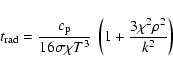
The radiative time scales based on ATLAS6 and PHOENIX Rosseland mean opacities are rather similar in the deeper layers while being very different in the optically thin regime. This emphasizes the great influence of molecular absorption which becomes important at cooler temperatures and which is not included in the ATLAS6 opacities. The radiative time scales from PHOENIX Rosseland and Planck opacities differ also significantly. Comparing the radiative time scales to a dynamical or convective time scale as given by the Brunt-Väisälä period leads us to expect that one gets a qualitatively different behavior depending on the treatment of the radiative transfer. We will see that models based on a frequency-independent Rosseland opacities show significant deviations from radiative equilibrium conditions. A more realistic treatment - in the optically thin regions more closely represented by the Planck mean opacities - results in an atmospheric structure closer to radiative equilibrium. In all cases, one expects an almost adiabatic structure in the deeper layers since the radiative relaxation time is much longer than the convective time scale.

Figure 4: Various characteristic time scales as a function of pressure in an M-dwarf model: Brunt-Väisälä period (solid), Kelvin-Helmholtz time scale (dashed), radiative relaxation time based on ATLAS6 Rosseland opacities (dotted), PHOENIX Rosseland (dashed-dotted), and PHOENIX Planck (triple-dot-dashed) opacities. A logarithmic Rosseland optical depth scale is indicated by the tick marks near the abscissa. The kink in the run of the Brunt-Väisälä period is located at the boundary between the convectively stable and unstable part of the model.

Open with DEXTER

3.1 A remark on thermal relaxation

RHD uses an explicit numerical scheme for advancing the solution in time. It is well known that in an explicit scheme the time step is limited to a fraction of the dynamical time scale, more precisely to the limit given by the Courant-Friedrichs-Levy stability condition. Together with the amount of available computer - and wallclock - time, this limits the time interval which can be covered by a 3D RHD model to about $10^4\mbox{\rm ~s}$ of stellar time. Figure 4 seemingly implies that it is impossible to obtain a thermally relaxed hydrodynamical model within this time interval since the Kelvin-Helmholtz time scale of the deeper layers is at least an order of magnitude larger. Contrary to the impression given in Fig. 4, in the multi-dimensional hydrodynamical simulations this does not pose a problem since the thermal relaxation of the model is not governed by the time scale for the exchange of energy as expressed by the Kelvin-Helmholtz time. In fact, the thermal evolution of the deeper layers of the RHD models is governed by the time scale for the exchange of mass in these layers which is much shorter (as quantified below, see Fig. 16). Due to the exponential run in density of the atmosphere the mass exchange consists primarily of the replacement of mass by fresh material stemming from deeper layers. In the hydrodynamical model it is ultimately fed into the computational domain at the lower boundary. The convective energy flux is the net effect of the energy transported by counteracting, opposing mass currents in and out of a test volume. The advective - as opposed to diffusive - nature of the mass transport leads to a situation where there can be a large imbalance in the energy content of the mass currents: the in-coming mass elements carry the energy (strictly speaking the specific entropy) of much deeper layers (in the hydrodynamical model the entropy at the lower boundary), while the out-going elements just carry the local energy density. This implies an energy flux much larger than the one close to equilibrium conditions. The system is driven much faster towards equilibrium than implied by the classical Kelvin-Helmholtz time scale, which assumes an energy flux as encountered close to equilibrium conditions.

We have argued from the perspective of our hydrodynamical models. But the fast thermal relaxation is driven by a physical mechanism implying that a real stellar convection zone does not operate any differently. Hence, we want to stress that to our understanding the thermal relaxation of a convective layer is generally not governed by the classical Kelvin-Helmholtz time scale but by the usually shorter time scale of mass exchange.

In the one-dimensional LHD models no mass exchange takes place and the convective energy flux is computed from MLT, in which convection is modeled as diffusion process. Under such circumstances the time scale of the thermal evolution of the convective layers is indeed comparable to the Kelvin-Helmholtz time scale as shown in Fig. 4. Of course, covering the time interval necessary for the slower thermal relaxation in a 1D model run poses no problems due to the largely reduced computational costs.

4 2D precursor models

Models C-2D and D-2D are 2D models (see Table 1) which were constructed to gain experience regarding the size of the computational domain and grid resolution. They are based on grey radiative transfer utilizing ATLAS6 opacities which do not include contributions of molecular lines. The choice of the ATLAS6 opacities was dictated by the lack of more realistic opacities during the initial phase of the project. From Fig. 4 one might readily conclude that their atmospheric structure will be dominated by convection since the radiative relaxation times in the atmosphere are long as compared to the dynamical time scale. Indeed, when starting from a temperature structure taken from a LHD model based on MLT, we find a rapid cooling of the originally radiatively stratified atmospheric layers by convective overshooting (see Fig. 5). Convection tends to transform the stratification into a purely adiabatic one since the radiative heating is too weak to keep the temperature close to the radiative equilibrium value. The transformation into an almost adiabatic stratification takes too long to be covered within the multi-dimensional hydrodynamical simulations. However, we conducted numerical experiments with LHD where an ad hoc velocity field mimicking the convective overshoot was put into the atmospheric regions which are formally stable according to the Schwarzschild criterion. The LHD models indicate that the asymptotic temperature profile tends to a fully adiabatic stratification.

Figure 5: Temporal evolution of the average temperature profile of model C-2D in steps of 5 ks showing a successive cooling of the layers around $\log P = 5.5$ (solid lines). For comparison a LHD model with $\ensuremath {\alpha _{{\rm MLT}}} =1.0$ is plotted (dash-dotted). All models are based on grey radiative transfer employing ATLAS6 opacities devoid of molecular contributions. All models have the same atmospheric parameters (  = 2770 K,  = 5.0). A logarithmic Rosseland optical depth scale is indicated by the tick marks near the abscissa.

Open with DEXTER

Due to the unrealistic opacities, the models cannot give a good representation of a real M-dwarf atmosphere. They are nevertheless interesting from a numerical point of view. The resolution of the less resolved model C-2D is already sufficient to represent the convective transport properties, in particular in the important transition region from convectively to radiatively dominated energy transport: after an initial relaxation phase we find in both models that the minimum temperature drops linearly with a rate of $\frac{{\rm d}T}{{\rm d}t}=-0.011\mbox{\rm ~K/s}$. Looking at further diagnostics at comparable instances during the secular evolution of the model runs we observe that RMS velocities are similar within a 20% level. The higher resolved model shows somewhat more small-scale features, and its downflows appear more concentrated. However, we are primarily interested in the balance of convective to radiative energy transport. The temperature drop rate is a convenient measure of the relative efficiency of both processes. Hence, we conclude from the similarity of the drop rates that the resolution of the less resolved model applied in 3D simulations is sufficient to model the transport properties of the convective flows.

Another conclusion which can be drawn from these models is that standard MLT models can give quite misleading predictions of the atmospheric temperature structure if the radiative relaxation time is long in comparison to convective time scales. In other words, one should be cautious when the coupling of the temperature structure to the radiative equilibrium temperature is so weak that overshoot of low amplitude happens essentially adiabatically. In the following we shall see that M-dwarf atmospheres are unlikely to exhibit such conditions.

5 3D models: Results and discussion

5.1 General flow structure

Figure 6 shows a typical snapshot of the emergent intensity during the temporal evolution of model B-3D. For comparison, Fig. 7 shows a similar snapshot from the solar run S-3D. Note, that the spatial and intensity scaling is very different in the reproductions, hence, only relative geometrical properties should be directly compared. The average relative RMS intensity contrast of the granular pattern amounts to 1.1% in the M-dwarf as opposed to 16% in the solar case. The first thing to note is that surface convection in an M-dwarf produces a granular pattern qualitatively resembling solar granulation: bright extended regions of upwelling material which are surrounded by dark concentrated lanes of downflowing material. The dark lanes form an interconnected network. Looking more closely, granules are less regularly delineated in M-dwarfs, the inter-granular lanes show a higher degree of variability in terms of their strength. A feature which is uncommon in the solar granulation pattern are the dark "knots'' (e.g. at $x=100\mbox{\rm ~km}$ and $y=230\mbox{\rm ~km}$ in Fig. 6) found in or attached to the inter-granular lanes. The knots are associated with strong downdrafts which carry a significant vertical component of angular momentum. The width of the inter-granular lanes to the typical granular size is smaller in M-dwarfs. Inspecting the velocity field (not shown) in vicinity of the continuum forming layers shows less pronounced size differences. This indicates that the relatively broader lanes in the solar case are the result of a stronger smoothing of the temperature field due to a more intense radiative energy exchange, i.e. the effective Peclét number of the flow is larger around optical depth unity in M-dwarfs.

	Figure 6: Typical snapshot of emergent intensity during the evolution of model B-3D. The intensity contrast amounts to $\delta I_{\rm rms}=1.2\%$ at this instant in time. Note, that the contrast of the intensity pattern in the graphics is enhanced with respect to its real appearance.
Open with DEXTER

	Figure 7: Like Fig. 6, but for the solar model S-3D. The intensity contrast amounts to $\delta I_{\rm rms}=16.7\%$ at this instant in time. Note, that for reproduction purposes spatial as well as intensity scale are altered in comparison to Fig. 6.
Open with DEXTER

The different magnitude of the intensity contrast already indicates that horizontal fluctuations of the thermodynamic quantities are small in M-dwarf atmospheres. Figure 8 shows the run of the relative temperature and pressure fluctuations in model A-3D. Plotted are long term temporal and horizontal rms averages. As we will argue later, the fluctuations in the higher atmosphere are likely to be overestimated in the model. But even taken at face value they are quite modest. The low level of fluctuations in the thermodynamic quantities is accompanied by small flow velocities, the maximum Mach number amounts to 6.5% in model A-3D. MLT models show that Mach numbers drop to even lower values as one goes to lower effective temperatures which are encountered in the regime of brown dwarfs. Our findings may have a direct bearing on the dust formation conditions in such objects. Our hydrodynamical simulations support the view that dust forming layers in cool main sequence objects experience only small variations around their mean thermodynamic state. This view is clearly at odds with the scenario discussed by Helling et al. (2001) who study the dust formation in turbulent brown dwarf atmospheres. Helling et al. assume thermodynamic fluctuations of order unity.

Figure 8: Relative horizontal temperature (solid) and pressure (dashed) fluctuations of model A-3D. The fluctuations in the region $\log P < 5$ are likely to be overestimated in the model, i.e. should be considered as upper limits. The dotted line indicates the approximate location of the Schwarzschild boundary. A logarithmic Rosseland optical depth scale is indicated by the tick marks near the abscissa.

Open with DEXTER

Another important feature, which distinguishes M-dwarf atmospheric conditions from solar ones, is the extent of the convective layers. As evident from Figs. 11 and 12, the convective motions reach much lower optical depth ( $\log\tau_{{\rm Rosseland}}$ $\approx$ -1.5) in the M-dwarf than in the Sun ( $\log\tau_{{\rm Rosseland}}\approx 0$). Two factors contribute to this behavior. The temperature gradient in non-grey radiative equilibrium is significantly steeper in the M-dwarf than in the Sun, presumably due to efficient cooling of the atmospheric layers by molecular lines. Furthermore, the ${\rm H}_2$ molecule formation reduces the adiabatic gradient in the M-dwarf atmosphere, while in the Sun the hydrogen recombination is essentially completed in subphotospheric layers. The different radiative and thermodynamic conditions favor the presence of convection in M-dwarf atmospheres.

In the deeper layers we observe the tendency - also known from solar simulations (see Stein & Nordlund 1998) - that the granular network of downflows decays into isolated downdrafts. Our models are rather shallow reaching only 2.3 pressure scale heights below optical depth unity. Thus we cannot follow the change of flow topology as far as has been done for solar models, but within the limited depth range comprised by our models we do not see indications of a qualitatively different behavior as found in the Sun.

5.2 Horizontal scales

In the following we shall discuss spatial power spectra of intensity and vertical velocity. Note, that in the Figs. 9 and 10 we display power per logarithmic wavenumber interval and not per unit wavenumber - the more common choice. This allows visually for a more direct identification of the power carrying scales. However (in humble respect of Kolmogorov's achievements), we labeled the power laws drawn for comparison with the familiar spectral index of power per unit wavenumber. The spectra are temporal averages over one to a few convective turn-over times and many convective cells, so that they are statistically representative.

Figure 9 shows a comparison of power spectra of the emergent intensity (more precisely: the intensity in the OBM continuum bin in vertical direction at the upper boundary of the computational volume) for the models A-3D, and B-3D as well as the solar model. Figure 10 shows a corresponding comparison of the vertical velocity component measured at the layer where its RMS value reaches the maximum. To facilitate a comparison between the M-dwarf models and the solar model, the solar model was arbitrarily scaled in power and wavenumber so that the maxima and position of the power distributions matched. For the M-dwarf models the hump in power at the highest wavenumbers is likely an artifact of an imperfect choice of parameters controlling the small scale dissipation and should be ignored.

Figure 9: Power spectrum of the emergent intensity pattern for model A-3D (solid), and B-3D (dashed), as well as the solar model S-3D (dotted). The spectrum of the solar model was scaled in power as well as wavenumber to match the peak of power in the M-dwarf models. Lines with slopes $\frac{{\rm d}P}{{\rm d}k}\propto k^{-5/3}$and $\frac{{\rm d}P}{{\rm d}k}\propto k^{-17/3}$ are shown for comparison with expectations from simplistic turbulence theory. The total relative intensity contrasts amount to $\delta I_{{\rm rms}}=$ 1.12% (A-3D), 1.12% (B-3D), and 16.2% (S-3D).

Open with DEXTER

	Figure 10: Power spectrum of the vertical velocity pattern, line styles as in Fig. 9. The solar power spectrum was scaled to match the peak of power of the M-dwarf models. The velocity pattern was taken from the layer where the RMS vertical velocity reaches its maximum, with absolute values of $v_{{\rm rms,max}}=$ 236 m s-1(A-3D), 241 m s-1 (B-3D), 2600 m s-1 (S-3D).
Open with DEXTER

Fluctuations in the Sun are an order of magnitude larger and had to be reduced accordingly in order to match the height of the maxima in the M-dwarf models, while the horizontal scale of the solar model had to be shrunk by a factor of 15. This factor closely corresponds to variation of the pressure scale height at the surface (factor 12.5) and follows the scaling found for hotter models by Freytag et al. (1997). Different from Freytag et al., we accounted for the change of the mean molecular weight of the stellar gas since the H₂ molecular formation leads to a significant increase in M-dwarf atmospheres. The peak power of the M-dwarf models is located at an absolute scale of 80 km for intensity and 63 km for velocity structures.

Comparing the width of the power distribution at 1 dex below peak level, the M-dwarf model B-3D displays a range of scales of 1.4 dex, the solar model of 1.1 dex. As is evident from the figures, the solar scale distribution is slightly but noticeably narrower. This might be traced back to the lower Péclet number of the plasma encountered at the surface of an M-dwarfs as opposed to solar conditions. The formation of small scale structures is more strongly suppressed by the radiation field under solar conditions, leading to an overall narrower power distribution. Model A-3D apparently lacks some larger scale power indicating that the computational box is somewhat too small in this case. However, since the total fluctuations are very similar in the models we conclude that the relevant structures are captured in model A-3D which serves as our standard model.

Towards high wavenumbers the M-dwarf spectra do not show a clear power law behavior. In any case, they cannot be fitted with a -5/3 slope, and are at best roughly compatible with a -17/3 slope. We would like to emphasize that despite the very different physical parameters of M-dwarf atmospheres this is qualitatively what was already found in solar models, and is at odds with expectations for homogeneous and isotropic turbulence. While smaller scales in the hydrodynamical models are definitely influenced by the artificial viscosity, it is still somewhat surprising that the asymptotic behavior in the Sun as well as in the M-dwarf is so similar despite their quite different characteristic flow speeds (i.e. Mach numbers). While our present models cannot make definite statements about the properties of small scale turbulence, a "non-Kolmogorov'' behavior cannot be ruled out neither. See Nordlund et al. (1997) for an in-depth discussion of this issue in a solar context.

5.3 Mean temperature stratification and corresponding effective mixing-length parameter

Figures 11-13 show a comparison of the thermal structure of our "best'' hydrodynamical model A-3D with standard 1D atmosphere models computed with LHD. Again, we point out that the treatment of the microphysics (equation of state and opacities) is equivalent between RHD and LHD models. Differences lie mainly in the dimensionality of the models - 3D versus 1D - and the related MLT treatment of the convective energy transport in LHD. In LHD effects of the turbulent pressure due to convective velocities computed from MLT are neglected. This approximation is well justified since the turbulent pressure - as found in the RHD simulations - nowhere exceeds 0.5% of the gas pressure.

Figure 11: Overview of the temperature-pressure relation of hydrodynamical model A-3D (solid) and three standard mixing-length model atmospheres (dash-dotted) with $\ensuremath {\alpha _{{\rm MLT}}} =1.0,1.5,2.0$. The $\ensuremath {\alpha _{{\rm MLT}}} =1.0$ model is the hottest at high pressure while it is coolest around $\log P$ = 5. A logarithmic Rosseland optical depth scale is indicated by the tick marks near the abscissa. All models have identical atmospheric parameters ( $\ensuremath{T_{{\rm eff}}} =2790\mbox{\rm~K}$, $\ensuremath{\log g} =5.0$, solar chemical composition). The dotted line indicates the location of the Schwarzschild boundary in the $\ensuremath {\alpha _{{\rm MLT}}} =1.0$ model. See Fig. 12 for an enlargement of the transition region from convective to radiative transport.

Open with DEXTER

	Figure 12: Temperature-pressure relations like in Fig. 11 but focusing on the transition region from convective to radiative energy transport. In this region the $\ensuremath {\alpha _{{\rm MLT}}} =1.0$ model is the coolest, $\ensuremath {\alpha _{{\rm MLT}}} =2.0$ the hottest mixing-length model.
Open with DEXTER

Figure 13: Entropy-pressure relation of hydrodynamical model A-3D (solid) and three standard mixing-length model atmospheres (dash-dotted) with $\ensuremath {\alpha _{{\rm MLT}}} =1.0,1.5,2.0$. The $\ensuremath {\alpha _{{\rm MLT}}} =1.0$ model has the largest entropy at high pressure while it has the lowest around $\log P=5$. The entropy level of material entering the computational box of hydrodynamical model A-3D at the lower boundary is indicated by the dashed line. All models have identical atmospheric parameters ( $\ensuremath{T_{{\rm eff}}} =2790\mbox{\rm~K}$, $\ensuremath{\log g} =5.0$, solar chemical composition).

Open with DEXTER

For the hydrodynamical model we have plotted in fact six different mean stratifications in the afore mentioned figures, each one a horizontal and temporal average over a 250 s time interval - comparable to the turn-over time of the convective cells. The statistical variations are so small that the profiles are virtually indistinguishable on the scale of the plots demonstrating again that we are dealing with atmospheres showing little temporal and horizontal fluctuations. Figure 11 shows that the mean thermal structure of the hydrodynamical model corresponds closely to those of mixing-length models. The mixing-length models themselves do not show a strong dependence on the mixing-length. In the deeper, convective layers small horizontal entropy fluctuations are sufficient to carry the convective flux, and the radiative energy transport is unimportant. Here the stratification has to follow essentially an adiabat in the pressure-temperature plane. The same reasoning holds for the hydrodynamical as well as MLT models. The situation is somewhat different in the radiative layers. By construction, the mixing-length models have to approach a temperature profile corresponding to radiative equilibrium conditions. Since the differences among the mixing-length models in the convective region are small the radiative equilibrium profiles are almost identical as well. In the hydrodynamical model the temperature of the higher atmospheric layers ( $\log P < 5.3$) is controlled by a competition of radiative heating and adiabatic cooling of material which overshoots into regions with formally stable entropy gradient $\frac{{\rm d}s}{{\rm d}P}<0$(see Fig. 13), and, analogously, the radiative cooling and adiabatic heating of downflowing material. The relative time scales involved in adiabatic and radiative temperature changes determine how the temperature will adjust between the upper extreme - the radiative equilibrium temperature - and the lower extreme - the temperature achieved during adiabatic expansion of a rising mass element in the higher atmosphere.

Obviously, in the present case, radiative processes dominate and the hydrodynamical model closely follows the radiative equilibrium temperature. As we have seen in the context of the hydrodynamical models adopting grey ATLAS6 opacities this is not necessarily so. In fact, we trace back the short radiative time scales (see Fig. 4) to the presence of molecular absorption which provides the close coupling of the stratification to the radiative equilibrium temperature. We speculate here that the situation might change significantly when one goes to metal poor objects. Convective velocities are likely not to be reduced as dramatically as the atmospheric opacities, shifting the relative importance towards adiabatic cooling. This might lead to a significant deviation from radiative equilibrium in the atmospheric layers of such objects. Indeed, for metal poor dwarfs at about solar effective temperatures such effects are found in hydrodynamical models (e.g. Asplund & Garcia Perez 2001).

Quantitatively, there are small differences in the thermal structure between the hydrodynamical model and the mixing-length models. As one can expect the differences are most pronounced in the transition region between convectively and radiatively dominated energy transport where the detailed balance between both processes decides about the resulting temperature profile. Figures 12 and 13 show that the hydrodynamical model has a mean thermal structure which is close to the profiles of the mixing-length models but cannot be matched exactly. This certainly comes not as a big surprise when one considers the simplistic nature of mixing-length theory. However, certain aspects of the hydrodynamical model can be matched by choosing a mixing-length model from the set which are parameterized by . This is most easily done considering the entropy since it emphasizes model differences (see Fig. 13). The entropy of inflowing material of the hydrodynamical model which we interpret as the entropy of material located in the deep almost perfectly adiabatically stratified part of the stellar envelope is matched best by a mixing-length model of $\ensuremath{\alpha_{{\rm MLT}}} ({\rm evo})=1.5$. In global stellar structure models the entropy of the envelope controls to some extent the radius of a star, making $\ensuremath{\alpha_{{\rm MLT}}} ({\rm evo})$ most relevant for evolutionary models - hence, our naming "evo''. For further justification and discussion of our interpretation see Steffen (1993) and Ludwig et al. (1999).

If one wants to match the entropy jump of the hydrodynamical model $\ensuremath{\alpha_{{\rm MLT}}} (\Delta s)=2.1$ provides the closest fit. The entropy jump is the entropy difference between the atmospheric entropy minimum and the asymptotic entropy of the deeper layers. The entropy jump provides a qualitative measure of the overall available convective driving, and in the present case also gives a match to the temperature gradient of the deeper photosphere with $\log_{10}\ensuremath{\tau_{{\rm ross}}} >-1$. The internal uncertainties in the determination of $\ensuremath{\alpha_{{\rm MLT}}} ({\rm evo})$ and $\ensuremath{\alpha_{{\rm MLT}}} (\Delta s)=2.1$ are small ($\approx$$\pm 0.05$) as estimated from the statistical fluctuations observed in the models. However, in the present M-dwarf model small deviations from equilibrium conditions determine the mixing-length parameters. This is a challenging situation for any numerical scheme, and we consider it possible that the actual calibration errors are dominated by related systematic uncertainties.

5.3.1 Importance of the MLT formulation

Throughout this paper mixing-length parameters are given with respect to the formulation of MLT according Mihalas (1978) (see Ludwig et al. 1999 for details of the implementation). The formulation of Mihalas is widely used, in particular in the context of stellar atmosphere work. But it is by far not the only MLT "dialect'' around. Another widely used formulation is the original one by Böhm-Vitense (1958) which is often encountered in the context of stellar evolution work. We would like to emphasize that generally the details in the MLT implementation have a direct and significant influence on the calibration of the mixing-length parameter. This is particularly true in the present case where convection penetrates far into optically thin regions. Typically it is the treatment of the radiative energy exchange of the convective elements in the optically thin limit that distinguishes the various MLT formulations. For enabling inter-comparison in other context, we like to mention that the MLT formulation in PHOENIX is similar but slightly different from the Mihalas formulation. However, test calculations have shown that numerical differences are negligible in the M-dwarf regime. Furthermore, in the ATLAS6 stellar atmosphere code the Mihalas formulation is implemented. MLT formulations as given by Kippenhahn & Weigert (1991) and Stix (1989) are identical to the Böhm-Vitense formulation.

Figure 14: Entropy-pressure relation of hydrodynamical model A-3D (solid) and standard mixing-length model atmospheres with $\ensuremath {\alpha _{{\rm MLT}}}$ = 1.5 based on two different formulations of MLT: Mihalas (1978) (dot-dashed) and Böhm-Vitense (1958) (dotted). Note, the significantly different entropy jumps in the MLT models employing the same mixing-length parameter. The entropy level of material entering the computational box of hydrodynamical model A-3D at the lower boundary is indicated by the dashed line. All models have identical atmospheric parameters ( $\ensuremath{T_{{\rm eff}}} =2790\mbox{\rm~K}$, $\ensuremath{\log g} =5.0$, solar chemical composition).

Open with DEXTER

Figure 14 shows a comparison of the entropy profiles of standard mixing-length models of the same $\ensuremath{\alpha_{{\rm MLT}}} =1.5$ based on the the Mihalas and Böhm-Vitense formulation. We concentrate on the entropy jump since it is sensitive to the convective transport in the optically thick and thin layers. The asymptotic entropy level of the deeper layers is largely controlled by the entropy change over the optically thick layers only. Mihalas and Böhm-Vitense formulation differ little here, implying the rather similar outcome. The formulations differ significantly in the optically thin layers. Clearly, the entropy jump comes out to be almost a factor of 2 larger in the Böhm-Vitense formulation! To reduce the entropy jump to a level comparable as obtained from the Mihalas formulation, one had to increase the mixing-length parameter noticeably. Again, this emphasizes that is only well defined with reference to a specific MLT formulation.

The Böhm-Vitense formulation assumes optically thick convective elements throughout. Their radiative energy exchange is described in diffusion approximation. It might be surprising that the entropy jump obtained from the Böhm-Vitense formulation is larger than from the Mihalas formulation which distinguishes between optically thick and thin elements. The optically thin elements loose (or gain) energy in a non-diffusive fashion. A larger entropy jump implies larger radiative losses of the convective elements. Intuitively, one would expect that a diffusive transport is rather inefficient, implying a smaller energy exchange and smaller entropy jump. However, Eq. (A.3) shows that the situation is reversed: the thermal adjustment time of convective elements becomes independent of their optical thickness in the optically thin limit, while the diffusion approximation predicts (inaccurately) a decrease of the adjustment time with decreasing optical thickness. Since the optical thickness becomes very small in the optically thin limit, the diffusion approximation underestimates the thermal relaxation time, and overestimates the radiative losses which leads to a larger entropy jump.

While it appears at first glance arbitrary which MLT formulation one chooses, Fig. 14 also shows that in the present case the formulation of Mihalas is perhaps superior to the formulation of Böhm-Vitense. The shape of the entropy profile of the Mihalas model resembles the result of the hydrodynamical model more closely. This comes at no surprise since the formulation of Mihalas considers optically thick and thin convective elements - i.e. better represents the actual situation. Of course, our choice of relating our to the formulation of Mihalas was motivated by this property.

5.3.2 Comparison to the Sun

It is interesting to compare equivalent mixing-length parameters derived for the thermal structure of the hydrodynamical models with other ones found in hotter objects, especially the Sun. Using the MLT formulation of Böhm-Vitense, Ludwig et al. (1999) found in a study of the convective efficiency based on 2D hydrodynamical models $\ensuremath{\alpha_{{\rm MLT}}} =1.6$for the Sun which has likely to be corrected to $\ensuremath{\alpha_{{\rm MLT}}} =1.8$ if one considers 3D models. In the Sun no distinction needed to be made between fitting the entropy jump or the asymptotic entropy. The solar mixing-length models match the photospheric entropy minimum found in the hydrodynamical models quite well. This is a consequence of the fact that convection does not reach very far up into optically thin regions. Together with the relatively large entropy jump which makes the exact value of the entropy minimum less important this leads to the "one $\ensuremath {\alpha _{{\rm MLT}}}$ fits both'' situation. Contrary to the situation in M-dwarfs differences between the Böhm-Vitense's and Mihalas' MLT formulation are small in the Sun, again, a consequence of the confinement of convection to optically thick regions. This allows us to inter-compare the mixing-length parameter obtained by Ludwig et al. (1999) for the Sun with the values derived here.

The mixing-length parameter of 1.8 for the Sun and 1.5 (matching the asymptotic entropy) or 2.1 (matching the entropy jump) for the M-dwarf are not vastly different, the solar value even falls within the range spanned by the M-dwarf values. In MLT the convective flux scales as the square of , hence we are considering a flux variation within a factor of 2 only. Convection is efficient in M-dwarfs in the sense that the whole envelope is almost adiabatically stratified. The convective energy transport process itself does not work much differently than in the solar case - taking the similar mixing-length parameters as a measure. The adiabatic behavior follows mostly from the reduction of the transported flux which can be accommodated with smaller horizontal entropy fluctuations. This ultimately leads to the smaller entropy jump which amounts to $\Delta s=7 \times 10^6\mbox{\rm ~erg/g/K}$, or only $\approx$$4\%$ of the solar entropy jump. This is remarkable since as evident from Fig. 13 about half of the entropy jump happens to take place in the optically thin region which is qualitatively different from the Sun. Moreover, the MLT captures surprisingly well the convective transport properties under such conditions.

We note that an extrapolation of the entropy jump as found by Ludwig et al. (1999) (their Fig. 4) for F-, G-, and K-dwarfs leads to a significant overestimation of the entropy jump for M-dwarfs. This means that the trend in the entropy jump found in hotter objects changes at some point when moving towards lower . This, again, is plausible because the dominant atmospheric opacity source as well as contributors to the specific heat change in the M-dwarf regime.

5.4 Synthetic broad band colors

   

Table 2: Synthetic broad band colors V-I, R-I in the Cousins system, as well as J-K, and J-H in the CIT system for the models displayed in Fig. 11. The effective temperature  $\ensuremath {T_{{\rm eff}}} ^\prime$ corresponds to the total flux as computed by the detailed spectral synthesis.

Model	$\ensuremath {T_{{\rm eff}}} ^\prime$	V-I	R-I	J-K	J-H
	[K]	[mag]	[mag]	[mag]	[mag]
RHD, A-3D	2754	3.651	1.974	0.749	0.455
LHD, $\ensuremath {\alpha _{{\rm MLT}}} =1.0$	2743	3.733	2.010	0.739	0.449
LHD, $\ensuremath{\alpha_{{\rm MLT}}} =1.5$	2744	3.701	1.996	0.746	0.452
LHD, $\ensuremath {\alpha _{{\rm MLT}}} =2.0$	2745	3.686	1.989	0.749	0.454

Table 2 provides synthetic optical and near-infrared colors for the models discussed before and shown in Fig. 11. The colors of the hydrodynamical model have been calculated from the average pressure-temperature structure. In the calculation of the colors the radiation field has been sampled with a resolution of 2 Å, i.e. the treatment of frequency dependence is different and more detailed than the OBM used in the models proper. Here we are concerned with the relative behavior among the models. For the V-I and J-K colors appreciable discrepancies exist between observations and model predictions by PHOENIX (" NEXTGEN'' model grid) in the -range $3600\mbox{\rm ~K} > \ensuremath{T_{{\rm eff}}} > 2300\mbox{\rm ~K}$(Chabrier et al. 2000; Allard et al. 2001). In V-I the offset amounts to $\approx$0.2-0.3 mag in the sense that the NEXTGEN models are too blue. In J-K the offset amounts to $\approx$0.2-0.5 mag depending on the source of water line opacity data used in the models. The treatment of the convective energy transport in the MLT framework - employing a standard of 1.0 - was suspected to be one possible reason for the discrepancy. Table 2 shows that a detailed treatment of convection does not remedy the situation. The difference between the V-I color of the hydrodynamical model to the LHD $\ensuremath {\alpha _{{\rm MLT}}} =1.0$amounts to 82 mmag only. Moreover, the hydrodynamical model is even bluer than the mixing-length model, i.e. when assuming the same differential behavior for models employing detailed radiative transfer, the discrepancy between theory and observations gets even slightly worse. As expected from the thermal structure $\ensuremath {\alpha _{{\rm MLT}}} =2.0$gives the closest match in color among the three LHD models.

Our results strengthen those of Allard et al. (2000) and Chabrier et al. (2000) who explain most of the visual discrepancy in terms of missing opacities. We would also like to emphasize that an optical color mismatch of this magnitude does not indicate a major shortcoming of the PHOENIX models. The V-band, which is likely to be responsible for the color mismatch, is formed high up in the atmosphere. The radiative energy flux in the V-band is a small fraction of the total radiative output of the star. Hence, the problem of the optical colors is related to a part of the atmosphere that is of minor importance for the overall energetics.

Similarly, the discrepancies between observed and predicted near-infrared colors cannot be traced back to an inadequate treatment of convection with MLT. Possible differences between MLT and hydrodynamical models amount to 10 mmag only.

Table 2 allows us to address a side point, namely the question of how the hydrodynamical model A-3D and the mixing-length models shown in Fig. 11 can have the same effective temperature (2790 K) despite the fact that the hydrodynamical model is almost always noticebly hotter than the mixing-length models. Indeed, when calculating the total flux within the detailed spectral synthesis the corresponding effective temperature $\ensuremath {T_{{\rm eff}}} ^\prime$ of the hydrodynamical model appears to be slightly ($\approx$ $10\mbox{\rm ~K}$) hotter than the one of the mixing-length models - with an offset to the nominal due to the more detailed treatment of the radiative transfer. We interpret this as an effect of the small remaining non-linearities when interchanging the averaging of the temperature-pressure structure with the solution of the radiative transfer. Strictly speaking, in order to determine the colors of the hydrodynamical model one must perform the detailed calculation of the 3D radiation field for many instances in time and had to average subsequently horizontally and temporally. However, in the present context, the smallness of the effects did not appear worth the dramatically increased computational effort.

5.5 Mean velocity and corresponding effective mixing-length parameter

Figure 15: Velocity-pressure relation of hydrodynamical model A-3D (solid) and five standard mixing-length model atmospheres (dash-dotted) with $\ensuremath {\alpha _{{\rm MLT}}} =1.0$ to 3.5 in steps of 0.5. The velocities of the mixing-length models increase monotonically with . For the hydrodynamical model RMS vertical velocities from six different temporal windows are plotted. A logarithmic Rosseland optical depth scale is indicated by the tick marks near the abscissa. All models have identical atmospheric parameters ( $\ensuremath{T_{{\rm eff}}} =2790\mbox{\rm~K}$, $\ensuremath{\log g} =5.0$, solar chemical composition).

Open with DEXTER

In the previous sections we discussed mixing-length parameters associated with the thermal properties of our hydrodynamical models. We now want to turn to a dynamical feature - the velocity profile. Figure 15 shows a comparison of velocities of hydrodynamical model A-3D with convective velocities from mixing-length models. In the case of the hydrodynamical model RMS fluctuations of the vertical velocity, for the mixing-length models the MLT convective velocity are displayed. Six different temporal windows (each 250 s in length) have been used for averaging the hydrodynamical data, showing noticable variations of the mean velocity particularly in the higher atmospheric layers. The velocity plateau in the uppermost layers is an artifact of the upper boundary condition which stipulates the same velocity at the boundary and the grid points next to the boundary. In order to match the convective velocities in the convectively unstable layers we find that $\ensuremath{\alpha_{{\rm MLT}}} (v)=3.5$ gives a reasonable match around the velocity maximum. The hydrodynamical model has the tendency to retain higher velocities towards smaller atmospheric pressure as compared to the MLT models. The behavior of the velocities towards high pressure shows a faster decline than the MLT models. The deeper hydrodynamical model B-3D (not shown) exhibits a similar velocity maximum as model A-3D but a decline which is not as fast. We conclude that the decline in model A-3D is to some extend influenced by the lower boundary condition and an asymptotic behavior towards high pressure closer to MLT predictions is likely.

The hydrodynamical model shows an appreciable amount of overshoot into the formally stable atmospheric regions. Of course, by construction, standard MLT is unable to make any predictions about velocity amplitudes there. Two different components contribute to the velocities in the higher atmosphere: one contribution are waves excited by the stochastical fluid motions in the deeper layers and travelling upwards, the other contributions are advective motions overshooting into the stably stratified layers (see also Ludwig & Nordlund 2000).

Qualitatively, we expect that velocity fluctuations $v^\prime$associated with advective motions decay with increasing distance from the Schwarzschild boundary, roughly $v^\prime \propto P^f$ where f is a positive parameter of order unity. For undamped sound waves we would expect a height dependence of roughly $v^\prime \propto P^{-\frac{1}{2}}$. This means that the relative importance of both contributions shifts from advection dominated motions to wave dominated motions with increasing height. If the wave motions are not strongly damped we would ultimately expect an increase of the velocity fluctuations with height. Indeed, according to Fig. 15 this is what we observe in our model. The wave motions mostly arise from standing waves - i.e. excited acoustic eigenmodes of the computational box. The detailed run of the velocity in the overshoot layers reflects the location of nodes and anti-nodes of the eigenmodes in vertical direction which explains the non-monotonic behavior of the atmospheric velocity amplitude.

The spectrum and the structure of the eigenmodes are to some extent determined by the geometry of the computational domain. This means that the velocities in the higher atmosphere where the velocity amplitude is wave dominated are model dependent and should not taken for real without skepticism. In the next sections we will even argue that the velocity amplitudes of the acoustic modes observed in our particular models are probably strongly influenced by the numerics, and in this sense are mostly artificial. In order to study the transport properties of the atmospheric velocity field we will try to filter out as much of the acoustic contribution to the velocity field as possible.

5.6 Atmospheric overshoot and transport time scales

Stellar atmospheres around $\ensuremath{T_{{\rm eff}}}\approx 2800\mbox{\rm ~K}$ are too hot to allow for a significant formation of dust grains. However, already at slightly cooler effective temperatures, grain formation sets in and dust grains become major opacity contributors, i.e. an important factor in determining the thermal structure of the atmosphere. In fact, the spectral energy distribution in the range of effective temperatures $2500\mbox{\rm ~K} \leq T \leq 1500\mbox{\rm ~K}$ is crucially linked to the distribution of dust grains in the atmosphere (Allard et al. 2000). The amount of dust which is present is determined by chemical condensation and evaporation processes as sources and sinks, as well as macroscopic transport processes which carry dust grains away from their sites of formation. In M-dwarf atmospheres the transport is dominated by two opposing processes: gravitational settling of dust grains and their mixing due to the presence of velocity fields, either related to convection or global circulations induced by rotation (T. Guillot 2000, private communication). In our models, no dust formation takes place but we nevertheless find it worthwhile to give a characterization of the atmospheric mixing due to convection and convective overshoot. This can give at least a first order approximation of how convective mixing might operate when dust is actually present. The basic question which we want to address is whether convective overshoot can provide enough mixing to prevent dust grains from being completely removed from the atmosphere by gravitational settling.

Formally, we are interested in a statistical representation of the mean transport properties of the convective velocity field in vertical direction. The horizontal advection of dust grains by the convective velocity field probably produces horizontal inhomogeneities in the dust distribution. We neglect these here since i) we are targeting at the application of our results in standard 1D stellar atmosphere models, ii) the horizontal inhomogeneities are small scale (the size of a convective cell), i.e. hardly observable and iii) the uncertainties in our understanding of the dust formation process itself perhaps limits the achievable accuracy anyway. In view of the last point we present a proxy of the convective mixing only, without trying to derive a detailed statistical description of the transport properties of the convective velocity field, i.e. extracting its effective transport coefficients (cf. Miesch et al. 2000, as an example of a more stringent treatment).

Figure 16: Mass exchange frequency as a function of pressure for various degrees of subsonic filtering. The solid curves from top to bottom correspond to no filtering, $v_{{\rm phase}}\leq 1.0,~ 0.5,~ 0.25\mbox{\rm~km~s}^{-1}$, respectively. The dashed line is an extrapolation towards the asymptotic behaviour corresponding to a complete removal of acoustic contributions. The dashed-dotted line depicts the dependence if one assumes a velocity field calculated from linear theory. A logarithmic Rosseland optical depth scale is indicated by the tick marks near the abscissa. The dotted line indicates the location of the Schwarzschild boundary.

Open with DEXTER

Figure 16 shows the mass exchange frequency  which provides an approximate measure of the convective mixing. We define this quantity as

$$\ensuremath{f_{\rm exchange}} (z) \equiv \frac{\langle F_{{\rm mass}}^{{\rm up}}\rangle(z)}{\langle m_{{\rm col}}\rangle(z)}$$ (2)

where $F_{{\rm mass}}^{{\rm up}}$ is the upward directed mass flux, $m_{{\rm col}}$ the mass column density, and z the geometrical height. $\langle.\rangle$ denotes temporal and horizontal averages. Note that the average total mass flux $\langle F_{{\rm mass}}\rangle$ vanishes

$$\langle F_{{\rm mass}}\rangle = \langle\rho u_{z}\rangle = ... ... mass}}^{{\rm up}} + F_{{\rm mass}}^{{\rm down}}\rangle = 0.$$ (3)

$\rho$ denotes the density, u_z the vertical velocity component. is the frequency with which the mass above a certain height z is replaced by the flux of fresh material from below. Mass conservation and quasi-steadiness demand that the upward directed mass flux from below is compensated by a downward directed flux from above. As long as the flow field is sufficiently disordered this mass exchange should also go hand in hand with mixing of material; in this way, can be interpreted as mixing frequency of atmospheric layers above a certain reference height z. The assumption of a disordered velocity field was checked qualitatively by studying the behaviour of passive tracer particles being advected with the flow. The definition of was motivated from our expectation that the amplitude of the velocity field would strongly decline with distance from the convectively unstable zone. Freytag et al. (1996) find in hydrodynamical models that the velocity amplitude due to convective overshoot declines exponentially with distance from the Schwarzschild boundary, and promote this result as a generic feature of overshoot. In such a situation, the mass flux in or out of a control volume is dominated by the flux through the surface closest to the convectively unstable region. This is the reason why we consider just one surface (or height) through which mass is transported.

As mentioned previously, the atmospheric velocity field has strong contributions of acoustic waves generated in the deeper layers of the models. From the comparison (not shown) of the hydrodynamical models A-3D and B-3D - which has a slightly greater extent in depth - we concluded that instabilities associated with the lower boundary condition contribute to the excitation of waves, i.e. the waves are mostly a numerical artifact. We could not trace down the responsable process, but the behavior was apparently related to the high degree of adiabaticity the stratification exhibits close to the lower boundary. In the Sun the boundary condition operated stably. Besides the numerical findings, from a purely theoretical point of view one would expect that the generation of acoustic energy is rather inefficient in a flow with as low a Mach number (few percent) as in the present case. Finally, it turns out that the Richardson number associated with the horizontal shear introduced by the acoustic modes in the atmosphere is not low enough to render the shear flow unstable. No small scale turbulence is induced by the waves and their oscillatory velocity fields do not contribute significantly to the mixing of material. Hence, we concluded that the wave contribution to the velocity field should be discarded if one wants to measure its mixing efficiency.

We therefore removed the contribution of waves before evaluating the average mass flux by subsonic filtering - a technique invented in the context of solar observations for cleaning images from "noise'' stemming from the 5 min oscillations (Title et al. 1989). In short, one considers a time sequence of images and removes features with horizontal phase speeds greater than a prescribed threshold. This is achieved by Fourier filtering of the spatial-temporal data in the k-$\omega$ domain. In our case we worked with 150 snapshots of the flow field sampled at 10 s time intervals. The total length of the sequence was long in comparison to the periods of the excited acoustic modes. For every depth layer we performed a 3D Fourier analysis (one temporal, two spatial dimensions) of the vertical mass flux. We selected velocity thresholds

$$v_{{\rm phase}} = \frac{\left\vert\omega\right\vert}{\left\ve... ...vec{k} \right\vert} = 1.0,~ 0.5,~ 0.25\mbox{\rm ~km~s}^{-1}.$$ (4)

With these specific choices of $v_{{\rm phase}}$ we tried to remove acoustic features which had phase speeds in the order of the sound speed without affecting the slow convective motions which have maximum velocities of about 0.25 km s^-1 (see Fig. 15). Note that the technique accounts only for the horizontal component of the phase speed. This means that e.g. purely radial oscillations could not be removed by this procedure. An improvement could, in principle, extend the filtering technique to four dimensions (one temporal, three spatial dimensions). But this would require a much higher computational effort, in particular since one would first have to determine a suitable set of basis functions for the representation of features in the vertical direction, where simple harmonic functions do not form a proper set of eigenfunctions. Luckily, the standard subsonic filtering worked well enough in our case so that we did not have to pursue this issue further.

Figure 16 shows the resulting mass exchange frequency  as a function of height (expressed in terms of the mean pressure) for our hydrodynamical model A-3D. Lowering the threshold  $v_{{\rm phase}}$ leads to a significant decrease of the mass exchange frequency in the atmospheric layers while the deeper layers remain essentially unaffected by the subsonic filtering. This again shows that the velocity field of the higher atmospheric layers stems primarily from wave motions. Only the lowest threshold of 0.25 km s^-1 starts to affect the deeper layers since also convective flow features reach such velocities. The dashed line in Fig. 16 indicates our extrapolation of what to expect in case of a perfect removal of the acoustic contribution. Its slope is given by the envelope of the sequence of curves for increasing degree of subsonic filtering. We want to emphasize that by the very nature of the problem the filtering procedure does not apply a small correction to the signal but removes even most of the original signal in some layers. Wave motions almost inevitably dominate the flow velocity above a certain atmospheric level. Large corrections as exhibited in Fig. 16 are to be expected, but do not pose particular problems so that we are confident about the filtering procedure.

As an additional check of our approach we calculated for an LHD mixing-length model with $\ensuremath {\alpha _{{\rm MLT}}} =2.0$ linear eigenmodes describing the growth of a perturbation under the action of the convective instability. $\ensuremath{\alpha_{{\rm MLT}}} =2$ was chosen since the model gave among the available mixing-length models the closest match to the thermal structure of the hydrodynamical model. As horizontal wavelength of the pertubation we chose the horizontal extent of model A-3D of 250 km, i.e. the largest horizontal wavelength which could be accomodated in this hydrodynamical model. Freytag et al. (1996) showed that the velocity field of convective eigenmodes gives a reasonable representation of the velocity field in the overshoot region as long as the horizontal wavelength is chosen in the vicinity of the actually present convective scales. The dash-dotted line in Fig. 16 shows the shape of associated with the linear eigenmode. The velocity amplitude was scaled to match the maximum of in the deeper layers of the hydrodynamical model. Besides a systematic shift the functional behavior predicted by the mode is quite similar to the one of the hydrodynamical simulation. Moreover, the time scale for the growth of the perturbation comes out to 120 s which is of the same order as the convective turn-over time scale. The similar rate of decline of in the atmospheric layers strengthens our confidence in the robustness of our extrapolation procedure. However, changing the horizontal wavelength of the perturbation within reasonable limits as well as experimenting with different background models did not improve the correspondence between linear modes and non-linear hydrodynamical model beyond the quality shown in Fig. 16.

Strictly speaking, the mixing frequency displayed in Fig. 16 is a lower limit since we removed all contributions associated with waves. However, the arguments given before make it very likely that the contributions of wave motions to the mixing are negligible: the Mach number of the flow is low, and the weak waves motions which may be excited are associated with little turbulence. Therefore we believe that the derived mixing efficiency is close to what is encountered in a real M-dwarf atmosphere.

What are the possible consequences of the exponential decline of the mixing time scale due to convective overshoot? Following the work of Rossow (1978), one arrives at an estimate of about $10^4\mbox{\rm ~s}$for the typical time scale of dust sedimentation in M-dwarf atmospheres. According to our hydrodynamical models the convective mixing could counteract the sedimentation up to a layer of about two pressure scale heights above the formally convectively unstable layers. The convective turn-over time scale is of the order of $10^2\mbox{\rm ~s}$. This is slow enough to allow for dust nucleation in the upper regions of the convective envelopes of M-dwarfs - provided that the thermodynamic conditions allow for nucleation in the first place. From these considerations we would expect that dust clouds in M-dwarf (and brown dwarf) atmospheres are confined to layers in the vicinity of the upper Schwarzschild boundary of the convective envelope.

6 Concluding remarks and outlook

We used elaborate 2D and 3D radiation-hydrodynamics simulations to study properties of convection on the surface of a prototypical late M-dwarf ( $\ensuremath{T_{{\rm eff}}}\approx 2800\mbox{\rm ~K}$, $\ensuremath{\log g} =5.0$, solar chemical composition). Despite the significant differences in the physical conditions encountered in the solar and an M-dwarf atmosphere we obtained the striking result that M-dwarf granulation does not look qualitatively different from what is familiar from the Sun (see Fig. 6). Quantitative differences (intensity contrast 1.1%, horizontal scales $\approx$ $80\mbox{\rm ~km}$, maximum RMS velocities $\approx$ $240\mbox{\rm ~m~s}^{-1}$, convective turn-over time scale $\approx$ $100\mbox{\rm ~s}$) remain within the expectations derived from mixing-length theory.

Connected to this basic finding is the - for practical purposes - perhaps most important result that the temperature structure of the higher atmospheric layers is determined by the condition of radiative equilibrium, and is not very much affected by processes usually not accounted for in standard stellar atmosphere models. Convective overshoot as well as energy transport by waves do not significantly affect the temperature structure outside of the region of convective instability. We expect that this finding also holds for main-sequence objects of higher effective temperature where radiation becomes relatively more important.

Answering the questions posed in the introduction we confirm that in late M-dwarfs mixing-length theory can be applied to obtain a realistic description of the convective energy transport in a 1D stellar atmosphere code, provided one can remove uncertainties related to the choice of the mixing-length parameter. If an independent calibration is available we expect that 1D atmosphere models allow reasonable accurate predictions (on a level as displayed in Fig. 13) of the atmospheric temperature structure and ultimately the stellar spectrum to be made. Effects on the stellar spectrum related to horizontal temperature inhomogeneities are expected to be very small in the M-dwarf studied here, primarily due to the small horizontal fluctuations of the thermodynamic variables. Even in the Sun - with the much higher temperature contrast present at its surface - effects related to horizontal temperature inhomogeneities are rather subtle (cf. Steffen & Ludwig 1999). We expect that 1D stellar atmosphere models provide an acceptable overall approximation to the spectrum of main-sequence objects between the Sun and late M-dwarfs. Only if one demands for a precision exceeding commonly adopted levels or desires to study effects in principle not included in standard model atmospheres (e.g. spectral line shifts and asymmetries), one has to go to more sophisticated modeling. We emphasize that this refers to objects at solar metallicity. For metal poor objects the situation is clearly different (see Asplund et al. 1999).

A downside of our findings is that we cannot trace back the remaining differences between theoretical and observed colors for M-dwarfs to shortcomings in the treatment of the convective energy transport. The resolution of the problem has to be found elsewhere, as pointed out earlier, deficiencies in the molecular opacities are still a possible option.

We are left with the problem of finding an adequate value of the mixing-length parameter to obtain a description of the vertical temperature run in the superadiabatic layers. In the present case we find a mixing-length parameter ($\Delta s$) = 2.1 which gives a match to the entropy jump and the temperature gradient of the deeper atmospheric layers (see Fig. 13). Despite perhaps the best value to be employed in stellar atmosphere calculations, for global stellar structure models a value of ($\Delta s$) = 1.5 would be more appropriate since it ensures to find the correct asymptotic entropy in the convective envelope which is important for obtaining the correct stellar radius. To complete the "zoo'' of mixing-length parameters, we get a value of (v) = 3.5 when matching the convective velocities predicted in our hydrodynamical models. We reiterate that all values are given with reference to the formulation of MLT by Mihalas (1978).

The various values of the mixing-length parameter point towards the deeper rooted problem that MLT can give a reasonable but not exact description of the average convective properties. Even calibrating one aspect does not ensure the overall correct functional form of, say, the temperature profile. We have seen that different formulations of MLT can give quite different functional dependencies. They offer the possibility to improve fits beyond the quality limited by fitting the mixing-length parameter only. For late M-dwarfs all this does not matter much since the differences of the atmospheric structure for various values of are small. However, we stress that this statement refers to cooler M-dwarfs on or close to the main-sequence. For pre-main-sequence (PMS) objects the situation is markedly different (Baraffe et al. 2002). There the specific choice of has a large impact on the resulting atmospheric structure. Work is underway to extend the present study into this regime which may also allow us to find the most suitable MLT formulation.

A result beyond the scope of classical model atmospheres is the derivation of a proxy of atmospheric mixing-time scales (see Fig. 16) due to convective overshoot. We find an exponential "leaking'' of the convective velocity field into the formally stably stratified layers. Depending on the exact criterion, overshooting extends the efficiently mixed regions about 2 pressure scale heights beyond the Schwarzschild boundary. We suggest that the mixing found in the $\ensuremath{T_{{\rm eff}}}\approx 2800\mbox{\rm ~K}$ model studied here, takes place in an analogous fashion in brown dwarfs, and provides the mixing which counteracts dust sedimentation. Hydrodynamical models can be used to address this problem more directly by performing simulations including the formation and transport of dust which we consider as an interesting challenge for the future.

Last but not least we would like to point out the two weakest points of our investigation. While the precision of the radiative transfer in the hydrodynamical calculations is sufficient to address the questions discussed here there is certainly room for improvement of the OBM to get an even closer agreement with detailed spectral synthesis calculations. Secondly, the models presented here are rather shallow. Improvements in the formulation of the lower boundary condition would perhaps allow the use of deeper computational domains, and would reduce the influence of the specific formulation of the lower boundary conditions.

Acknowledgements

The authors are indebted to Isabelle Baraffe and Gilles Chabrier for their supportive enthusiasm during the course of the project, and their scientific input during many discussions. HGL would like to thank Åke Nordlund and Robert Stein for making available a version of their hydrodynamical atmosphere code. PHH acknowledges support by "Pôle Scientifique de Modélisation Numérique'' (PSMN) at the École Normale Supérieure de Lyon, NSF grants AST-9720704 and AST-0086246, NASA grants NAG5-8425, NAG5-9222, as well as NASA/JPL grant 961582 to the University of Georgia (UGA), Athens. The calculations presented in this paper were performed on machines operated by the PSMN, on the NEC-SX5 at the "Institut du Développement et des Ressources en Informatique Scientifique'' (IDRIS), Paris, on the IBM SP2 of the UGA UCNS, on the IBM SP "Blue Horizon'' of the San Diego Supercomputer Center (SDSC) with support from the National Science Foundation, and on the IBM SP of the NERSC with support from the US Department of Energy. We thank all these institutions for a generous allocation of computer time.

Appendix A: Computation of the characteristic time scales

The radiative time scales shown in Fig. 4 were evaluated in Eddington approximation (see e.g. Edwards 1990) according

$$t_{{\rm rad}} = \frac{\ensuremath{c_{{\rm p}}} }{16\sigma\chi T^3} ~ \left( 1+\frac{3\chi^2\rho^2}{k^2}\right)$$ (A.1)

( denotes the specific heat at constant pressure, $\sigma$Stefan-Boltzmann's constant, $\chi$ opacity, T temperature, $\rho$mass density, k wavenumber of the disturbance). We assumed that the geometrical size of a thermal disturbance is the local pressure scale height  , hence

$$k = \frac{2\pi}{\ensuremath{H_{{\rm P}}} }\cdot$$ (A.2)

Introducing the optical size of the disturbance $\tau_{{\rm dis}}\equiv\chi\rho\ensuremath{H_{{\rm P}}}$ Eq. (A.1) can be written as

$$t_{{\rm rad}} = \frac{\ensuremath{c_{{\rm p}}} }{16\sigma\chi... ...} ~ \left( 1+\frac{3}{4\pi^2}~\tau_{{\rm dis}}^2\right)\cdot$$ (A.3)

Relation (A.3) shows that in the optically thin limit $\tau_{{\rm dis}}\ll 1$ the radiative relaxation time is independent of $\tau_{{\rm dis}}$, and in the optically thick limit $\tau_{{\rm dis}}\gg 1$ scales quadratically with $\tau_{{\rm dis}}$. Equations (A.1) and (A.3) describe the decay of a Fourier mode in an infinite isothermal atmosphere, i.e. make very idealizing assumptions. Our choice of of the local pressure scale height as size of the perturbation is somewhat arbitrary. Hence, the reader should take $t_{{\rm rad}}$ as depicted in Fig. 4 as order of magnitude estimates.

The (adiabatic) Brunt-Väisälä period  $t_{{\rm BV}}$ was calculated according

$$t_{{\rm BV}}=\frac{2\pi}{\sqrt{\left\vert\omega_{{\rm BV}}^2\... ...uremath{H_{{\rm P}}} }\left( \nabla_{{\rm ad}}-\nabla \right).$$ (A.4)

( $\delta\equiv -\left(\frac{\partial \ln\rho}{\partial \ln T}\right)_{\rm P}$ denotes the thermal expansion coefficient at constant pressure, ggravitational acceleration, $\nabla_{{\rm ad}}$ the adiabatic, and $\nabla$ the actual temperature gradient of the atmosphere). The local Kelvin-Helmholtz time scale  $t_{{\rm KH}}$ was evaluated according

$$t_{{\rm KH}} = \frac{P\ensuremath{c_{{\rm p}}} T}{g \sigma\ensuremath{T_{{\rm eff}}} ^4}$$ (A.5)

(P denotes the gas pressure) under the assumption that the overall energy content of a mass column is dominated by its thermal energy content.

References

 
• Allard, F., Hauschildt, P. H., Alexander, D., Tamanai, A., & Schweitzer, A. 2001, ApJ, 556, 357 In the text NASA ADS  
• Allard, F., & Hauschildt, P. H. 1995, ApJ, 445, 433 In the text NASA ADS  
• Allard, F., Hauschildt, P. H., Alexander, D. R., & Starrfield, S. 1997, ARA&A, 35, 137 In the text NASA ADS  
• Allard, F., Hauschildt, P. H., & Schwenke, D. 2000, ApJ, 540, 1005 In the text NASA ADS  
• Asplund, M., & Garcia Perez, A. E. 2001, A&A, 372, 601 In the text NASA ADS  
• Asplund, M., Ludwig, H.-G., Nordlund, Å., & Stein, R. 2000, A&A, 359, 669 In the text NASA ADS  
• Asplund, M., Nordlund, Å., Trampedach, R., & Stein, R. F. 1999, A&A, 346, L17 In the text NASA ADS  
• Baraffe, I., Chabrier, G., Allard, F., & Hauschildt, P. H. 2002, A&A, 382, 563 In the text NASA ADS  
• Böhm-Vitense, E. 1958, Zs. f. Ap., 46, 108 In the text  
• Brett, J. M. 1995, A&A, 295, 736 In the text NASA ADS  
• Chabrier, G., Baraffe, I., Allard, F., & Hauschildt, P. H. 2000, ApJ, 542, 464 In the text NASA ADS  
• Edwards, J. 1990, MNRAS, 242, 224 In the text NASA ADS  
• Freytag, B., Holweger, H., Steffen, M., & Ludwig, H.-G. 1997, in Science with the VLT Interferometer, ed. F. Paresce (Springer), 316 In the text  
• Freytag, B., Ludwig, H.-G., & Steffen, M. 1996, A&A, 313, 397 In the text  
• Gustafsson, B., Bell, R., Eriksson, K., & Nordlund, Å. 1975, A&A, 42, 407 In the text NASA ADS  
• Hauschildt, P. H., & Baron, E. 1999, J. Comp. Appl. Math., 102, 41 In the text  
• Helling, C., Oevermann, M., Lüttke, M., Klein, R., & Sedlmayr, E. 2001, A&A, 376, 194 In the text NASA ADS  
• Kippenhahn, R., & Weigert, A. 1991, Stellar Structure and Evolution (Springer Verlag) In the text  
• Kurucz, R. L. 1979, ApJS, 40, 1 In the text NASA ADS  
• Ludwig, H.-G., Freytag, B., & Steffen, M. 1999, A&A, 346, 111 In the text NASA ADS  
• Ludwig, H.-G., Jordan, S., & Steffen, M. 1994, A&A, 284, 105 In the text NASA ADS  
• Ludwig, H.-G., & Nordlund, Å. 2000, in Pacific Rim Conf. on Stellar Astrophysics, ed. K. Cheng, H. Chau, & K. Chan (Kluwer Academic Publishers), 37 In the text  
• Miesch, M. S., Brandenburg, A., & Zweibel, E. G. 2000, Phys. Rev. E, 61, 457 In the text  
• Mihalas, D. 1978, Stellar Atmospheres (Freeman and Company) In the text  
• Nordlund, Å. 1982, A&A, 107, 1 In the text NASA ADS  
• Nordlund, Å., & Dravins, D. 1990, A&A, 228, 155 In the text NASA ADS  
• Nordlund, Å., Spruit, H., Ludwig, H.-G., & Trampedach, R. 1997, A&A, 328, 229 In the text NASA ADS  
• Rossow, R. W. 1978, Icarus, 36, 1 In the text NASA ADS  
• Steffen, M. 1993, in Inside the stars, ed. W. Weiss, & A. Baglin, ASP Conf. Ser., 40, 300 In the text  
• Steffen, M., & Freytag, B. 1991, Rev. Mod. Astron., 4, 43 In the text  
• Steffen, M., & Ludwig, H.-G. 1999, in Stellar Structure: Theory and Test of Connective Energy Transport, ASP Conf. Ser., 173, 217 In the text  
• Stein, R. F., & Nordlund, Å. 1998, ApJ, 499, 914 In the text NASA ADS  
• Stix, M. 1989, The Sun (Springer Verlag) In the text  
• Title, A. M., Tarbell, T. D., Topka, K. P., Ferguson, S. H., & Shine, R. A. 1989, ApJ, 336, 475 In the text NASA ADS