A&A 394, 1039-1056 (2002)
DOI: 10.1051/0004-6361:20021176
New results on source and diffusion
spectral features of Galactic cosmic rays: I B/C ratio
D. Maurin 1 - R. Taillet 1,2 - F. Donato 3
1 - Laboratoire de Physique Théorique LAPTH, 74941 Annecy-le-Vieux, France
2 - Université de Savoie, 73011 Chambéry, France
3 - Università degli Studi di Torino and INFN,
Torino, Italy
Received 18 June 2002 / Accepted 29 July 2002
Abstract
In a previous study (Maurin et al. 2001), we explored
the set of parameters describing diffusive propagation of cosmic rays
(galactic convection, reacceleration, halo thickness, spectral index and
normalization of the diffusion coefficient), and we identified those
giving a good fit to the measured B/C ratio.
This study is now extended to take into
account a sixth free parameter, namely the spectral index of sources.
We use an updated version of our code where the reacceleration
term comes from standard minimal reacceleration models.
The goal of this paper is to present a general view of the evolution
of the goodness of fit to B/C data with the propagation parameters.
In particular, we find that, unlike the well accepted
picture, and in accordance with
our previous study, a Kolmogorov-like power spectrum for diffusion
is strongly disfavored. Rather, the  analysis points towards
 along with source spectra
index
along with source spectra
index  2.0.
Two distinct energy dependences are used for the source spectra:
the usual power-law in rigidity and a law modified
at low energy, the second choice being only slightly preferred.
We also show that the results are not much affected by a different
choice for the diffusion scheme.
Finally, we compare our findings to recent works, using other propagation models.
This study will be further refined in a
companion paper, focusing on the fluxes of cosmic ray nuclei.
2.0.
Two distinct energy dependences are used for the source spectra:
the usual power-law in rigidity and a law modified
at low energy, the second choice being only slightly preferred.
We also show that the results are not much affected by a different
choice for the diffusion scheme.
Finally, we compare our findings to recent works, using other propagation models.
This study will be further refined in a
companion paper, focusing on the fluxes of cosmic ray nuclei.
Key words: ISM: cosmic rays
Cosmic rays detected on Earth with kinetic energies per nucleon
from 100 MeV/nuc to 100 GeV/nuc were most probably
produced by the acceleration of a low energy galactic population of
nuclei, followed by diffusion in the turbulent magnetic field.
The acceleration process and the diffusion process have a magnetic
origin, so that they should depend on rigidity.
The rigidity dependence of the diffusion coefficient is given by
quasi-linear theory as
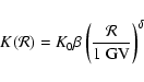 |
(1) |
where the parameters K0 and  should ideally be given by the
small-scale structure of the magnetic field responsible for the
diffusion. As this structure is not well observed, some
theoretical assumptions must be made in order to predict .
As regards the spectrum just after acceleration, the situation is far
from clear, as it depends on the details of the acceleration process.
Several models give a power-law distribution
(e.g. Berezhko et al. 1994; Gieseler et al. 2000)
should ideally be given by the
small-scale structure of the magnetic field responsible for the
diffusion. As this structure is not well observed, some
theoretical assumptions must be made in order to predict .
As regards the spectrum just after acceleration, the situation is far
from clear, as it depends on the details of the acceleration process.
Several models give a power-law distribution
(e.g. Berezhko et al. 1994; Gieseler et al. 2000)
 |
(2) |
with a definite value for  which depends on the model.
Most analyses of cosmic ray nuclei data assume given power-laws for
the diffusion and acceleration energy dependence, so that the
results partially reflect certain theoretical a priori.
In this work, we try to avoid this bias by determining the quantities
and
directly from the data, in particular B/C, for
reasons exposed below.
The paper is organized as follows. We first recall the main features
of our diffusion model. As a few modifications have been made since previous works,
Sect. 3 is devoted to their description and justification.
Then, the analysis method is described in Sect. 4 and the
results are shown and discussed in Sect. 5;
a comparison is eventually made with other similar works in Sect. 6.
This paper and its companion (Donato et al. in preparation) use
the same description of cosmic ray propagation as our previous analyses
(Maurin et al. 2001; Donato et al. 2001; Donato et al. 2002; Barrau et al. 2002; Maurin et al. 2002).
Particles are accelerated in a thin galactic disk, from which they
diffuse in a larger volume. When they cross the disk, they may
interact with interstellar matter, which leads to nuclear reactions
(spallations) - changing their elemental and isotopic composition - and
to energy losses. Interaction with Alfvén waves in the disk also
leads to diffusive reacceleration.
The reader is referred to Maurin et al. (2001) - hereafter
Paper I - for all details, i.e. geometry and
solutions of our two zone/three-dimensional diffusive model, nuclear parameters (nuclear grid
and cross sections), energy losses terms (adiabatic, ionization and
Coulomb losses), solar modulation scheme (force-field),
as well as general description of the procedure involved in our
fits to data (selection of a set of parameters,
test comparison
to data). In particular, though some inputs are modified (see
next section), the final equation describing cosmic ray equilibrium
is formally equivalent to that of Paper I (see Eq. (A13)):
it is a second order differential equation in energy solved with
the Crank-Nicholson approach (see Donato et al. 2001, Appendix B - hereafter
Paper II).
Finally, a schematic view of our diffusion model is presented
in Barrau et al. (2002) and Fig. 1 (see next section) summarizes
the algorithm of our propagation code.
Some aspects of this model are formally unrealistic.
First, the distribution of interstellar matter has a very simple
structure: it does not take into account a possible z distribution
inside the disk (thin disk approximation is used instead), nor radial and
angular dependence in the galactic plane.
The orthoradial  dependence would even be more important from an
accurate description of the magnetic fields and the ensuing diffusion,
as flux tubes are likely to be present along the spiral arms.
However, this is not crucial as we are interested in
effective quantities (diffusion coefficient and interstellar density)
but not in giving them a "microscopic'' explanation.
This is why we chose to use a universal
form of the diffusion coefficient, with the same value in the whole
Galaxy.
Finally, it is known that a fully realistic model has to take into account
interactions between cosmic ray pressure, gas and magnetic pressure,
i.e. magnetohydrodynamics.
dependence would even be more important from an
accurate description of the magnetic fields and the ensuing diffusion,
as flux tubes are likely to be present along the spiral arms.
However, this is not crucial as we are interested in
effective quantities (diffusion coefficient and interstellar density)
but not in giving them a "microscopic'' explanation.
This is why we chose to use a universal
form of the diffusion coefficient, with the same value in the whole
Galaxy.
Finally, it is known that a fully realistic model has to take into account
interactions between cosmic ray pressure, gas and magnetic pressure,
i.e. magnetohydrodynamics.
The semi-analytical diffusion approach should be thought of as an intermediate
step between leaky box approaches and magnetohydrodynamics
simulations and is actually justified by these two very approaches:
the first showed that the local abundances of charged nuclei can be roughly
described by two phenomenological coefficients - the escape length
and the interstellar gas density in the box.
The second hints at the fact that
the propagation models such as the one used here are well suited
for the description of cosmic ray physics.
However, it is difficult to conclude whether these parameters are valid for
other kinds of cosmic rays ( ,
,
 ,
nuclei induced
,
nuclei induced  -ray production)
and whether they are either meaningful but valid
only locally on a few kpc scale (i.e. not in the whole Galaxy -
see as an illustration Breitschwerdt et al. 2002),
or meaningless but phenomenologically valid as an average
description of more subtle phenomena (see as an example the
discussion of the Alfvénic speed in Sect. 6.3.4).
-ray production)
and whether they are either meaningful but valid
only locally on a few kpc scale (i.e. not in the whole Galaxy -
see as an illustration Breitschwerdt et al. 2002),
or meaningless but phenomenologically valid as an average
description of more subtle phenomena (see as an example the
discussion of the Alfvénic speed in Sect. 6.3.4).
3 New settings
Only a few ingredients differ from our previous analysis (Paper I). The reason
for these few changes is twofold: first, we attempt to use a better motivated
form of the reacceleration term; second, as the real value of the exponent
in the source power-law cannot be firmly established from acceleration
models - the latter being seemingly different from what is naively
deduced from direct spectra measurements -, it becomes a free parameter
in the present analysis.
3.1 Transport of cosmic rays
The starting point of all cosmic ray data analysis is the transport equation.
As emphasized in Berezinskii et al. (1990), a diffusion-like
equation was first obtained phenomenologically.
Afterwards, the kinetic theory
approach provided grounds for a consistent derivation.
This transport equation reads:
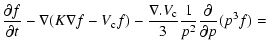 |
|
|
(3) |
 |
|
|
|
In this equation,
 is the phase space
distribution, K is the spatial diffusion coefficient,
is the phase space
distribution, K is the spatial diffusion coefficient,
 is
the momentum diffusion coefficient;
both are related to the diffusive nature of the process. Finally
is
the momentum diffusion coefficient;
both are related to the diffusive nature of the process. Finally  is the velocity describing the convective transport of cosmic rays
away from the galactic plane.
Actually, the full equation of cosmic ray transport includes
other terms, such as catastrophic and spontaneous
losses, secondary spallative contributions and continuous energy losses
(coulombian and ionization losses). These were taken into account as
described in detail in Paper I, to which the reader is referred for a complete description
and references. They will not be further discussed here.
is the velocity describing the convective transport of cosmic rays
away from the galactic plane.
Actually, the full equation of cosmic ray transport includes
other terms, such as catastrophic and spontaneous
losses, secondary spallative contributions and continuous energy losses
(coulombian and ionization losses). These were taken into account as
described in detail in Paper I, to which the reader is referred for a complete description
and references. They will not be further discussed here.
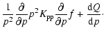
This equation can be rewritten using the cosmic ray differential
density
 .
As the momentum distribution function is normalized
to the total cosmic ray number density (
.
As the momentum distribution function is normalized
to the total cosmic ray number density (
 ),
we have
),
we have
 to finally obtain
 |
|
|
(4) |
![$\displaystyle \frac{\partial}{\partial E}\left[
-\frac{(1+\beta^2)}{E}K_{\rm pp}\;N(E)
+ \beta^2 K_{\rm pp}\frac{\partial N(E)}{\partial E}
\right] + Q(E);$](/articles/aa/full/2002/42/aa2811/img63.gif) |
|
|
|
with
 |
(5) |
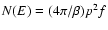
In this paper,
will be taken from the quasi-linear theory (see below).
From a theoretical point of view, the most natural choice for the
energy dependence of the source term seems to be a power-law in rigidity
(or momentum) for
 .
This translates into
.
This translates into
 in our set of
equations (see Eqs. (4) and (5) above). Several different forms
were used in the past because of the lack of strong evidence from
observed spectra (see for example Engelmann et al. 1985; Engelmann
et al. 1990). In particular, our previous analysis allowed only a rigidity
dependence
in our set of
equations (see Eqs. (4) and (5) above). Several different forms
were used in the past because of the lack of strong evidence from
observed spectra (see for example Engelmann et al. 1985; Engelmann
et al. 1990). In particular, our previous analysis allowed only a rigidity
dependence
 (for the special case
 ).
These two forms differ only at low energy and we chose to keep them
both to estimate their effect on our results. As we show below, it is
quite small.
).
These two forms differ only at low energy and we chose to keep them
both to estimate their effect on our results. As we show below, it is
quite small.
Finally, different diffusion schemes lead to different forms for the
energy dependence of the diffusion coefficient and the reacceleration
term.
Several aspects of the diffusion process are treated in Schlickeiser (2002), and we considered three alternative possibilities:
(i) Slab Alfven wave turbulence, with
 and
and
 ,
(ii) Isotropic fast magnetosonic wave turbulence, with
,
(ii) Isotropic fast magnetosonic wave turbulence, with
 and
and
 ,
and (iii) mixture of the two last cases,
,
and (iii) mixture of the two last cases,
 and
and
 .
.
All results will be presented with the case (i), except in the
specific discussion in Sect. 5.5.
3.2 Summary: Updates of Paper I's formulae
The only changes with our previous study are
- Eq. (19) of Paper I is replaced by
 |
(6) |
where
 |
(7) |
- Eq. (A13) of Paper I (second order differential equation to solve)
reads now - we use the same notations -
 |
(8) |
with
 |
(9) |
In our model,
 ,
but it has to be kept in mind that a possible
reinterpretation of
,
but it has to be kept in mind that a possible
reinterpretation of  is always possible (see Sect. 6)
as long as
is always possible (see Sect. 6)
as long as
 (this condition is necessary for the solution to be valid).
- As regards the source spectra, two forms
(hereafter type (a) and (b)) are used instead of Eq. (9) of Paper I
| a- Q(E) |
 |
 |
(10) |
| b- Q(E) |
|
 |
(11) |
where R is the rigidity and
a universal slope of
spectra for all nuclei heavier than helium.
4 Runs and selection method
The analysis presented here is the natural continuation
of the work presented in Paper I.
It is more general and it encompasses
its results as a five-dimensional subset of the six-dimensional
space scanned here.
The six parameters of this study are: the spectral index of sources
,
the normalization K0 and spectral index
of the diffusion
coefficient, the height of the diffusive halo L, the Galactic convective
wind speed
and the Alfvénic speed .
They are included in our code as follows (see Fig. 1 for a
sketch of the procedure): for a given set of parameters,
source abundances of all nuclei (i.e. primaries and mixed
nuclei) are adjusted so that the propagated
top of atmosphere fluxes agree with the data at 10.6 GeV/nuc (see Paper I).
We remind that for B/C ratio, we checked that starting the evaluation of
fluxes from Sulfur is sufficient (heavier nuclei do not contribute
significantly to this ratio).
![\begin{figure}
\par\includegraphics*[width=12cm,clip]{ms2811f1.eps}\end{figure}](/articles/aa/full/2002/42/aa2811/Timg80.gif) |
Figure 1:
Diagrammatic representation of the various steps of the
propagation code. |
| Open with DEXTER |
Top of atmosphere fluxes are deduced from
interstellar fluxes using the force field
modulation scheme (see Paper I
and references therein).
The resulting B/C spectrum is then compared to the data (see below)
and a
is computed for the chosen set of parameters.
This procedure is very time consuming. Even when the location of
minima in the six-dimensional parameter space are known,
more than
 configurations are needed to have a good sampling
of the regions of interest, for a given form of the source term energy
dependence.
configurations are needed to have a good sampling
of the regions of interest, for a given form of the source term energy
dependence.
4.2  criterion of goodness
As in our previous analysis, we have computed the quantity
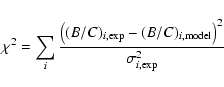 |
(12) |
where the sum runs over 26 experimental values from HEAO-3 (Engelmann et al. 1990)
with energies ranging from 620 MeV/nuc to 35 GeV/nuc (as in Paper I).
In general, if the experimental set-up is such that the measured (experimental)
values differ from the "real" values by a quantity of zero mean
(non biased) with a given probability distribution, then the value
of
gives a quantitative estimate of the probability that
the model is appropriate to describe the data.
However, this condition is probably not fulfilled for
HEAO-3, as for some measured quantity,
the quoted errors
 are much
smaller (e.g. oxygen fluxes) or much larger (e.g.
sub-Fe/Fe ratio) than the dispersion of data itself.
For this reason, it is meaningless to associate a likelihood to given
values.
Instead, in Paper I we decided that models giving
less
than some value
are much
smaller (e.g. oxygen fluxes) or much larger (e.g.
sub-Fe/Fe ratio) than the dispersion of data itself.
For this reason, it is meaningless to associate a likelihood to given
values.
Instead, in Paper I we decided that models giving
less
than some value  were "good fits" while the others were
"poor fits''.
In this paper, no cut is applied and all the models, whatever the value
of ,
are shown in the figures.
were "good fits" while the others were
"poor fits''.
In this paper, no cut is applied and all the models, whatever the value
of ,
are shown in the figures.
5 Results
5.1 Subset 1:
Fixed measured spectral index
 2.8
2.8
In this section we present the results obtained for source spectra of
the form
and diffusion coefficient
 .
At sufficiently high energies, spallations and
energetic changes are irrelevant and the measured fluxes can be
considered as a mere result of acceleration and diffusion
(see for example Maurin et al. 2002).
In this case,
the observed spectrum is proportional to
.
At sufficiently high energies, spallations and
energetic changes are irrelevant and the measured fluxes can be
considered as a mere result of acceleration and diffusion
(see for example Maurin et al. 2002).
In this case,
the observed spectrum is proportional to
 with
with
 .
In this section, we focus on the situation
.
In this section, we focus on the situation
 ,
corresponding to the spectral index of the measured
Boron progenitor fluxes.
Actually, Wiebel-Sooth et al. (1998)
analysed data from several experiments and derived smaller values.
In Paper I, we found that the Oxygen flux measured by HEAO-3
would be more compatible with our diffusion model for a higher ,
namely 2.8 instead of 2.68.
Anyway, we are more interested in the trends in the variation of
other parameters for a fixed value of
than in this precise
numerical value.
The other cases will be treated in the following sections.
,
corresponding to the spectral index of the measured
Boron progenitor fluxes.
Actually, Wiebel-Sooth et al. (1998)
analysed data from several experiments and derived smaller values.
In Paper I, we found that the Oxygen flux measured by HEAO-3
would be more compatible with our diffusion model for a higher ,
namely 2.8 instead of 2.68.
Anyway, we are more interested in the trends in the variation of
other parameters for a fixed value of
than in this precise
numerical value.
The other cases will be treated in the following sections.
We also set the halo thickness L to 6 kpc, leaving us with
four free parameters (,
K0,
and ).
All curves depicted in Fig. 2 correspond to one-dimensional
cuts through the absolute
minimum (for a given ,
the
three different cuts justify the fact that we are located in a minimum).
In the upper panel of Fig. 2, we plot the values of the as a function of K0/L, for different values of
(and the corresponding
 ).
).
![\begin{figure}
\par\includegraphics*[width=11.5cm,clip]{ms2811f2.eps}\end{figure}](/articles/aa/full/2002/42/aa2811/Timg90.gif) |
Figure 2:
Evolution of the
value for various combination
of parameters.
All curves are for type (a) spectra (
 )
with )
with
 and the halo size is fixed to L=6 kpc.
Each curve shows one-dimensional cuts in the K0/L (upper panel),
(left
lower panel)
or
(right lower panel) direction of the 3-dimensional
hyper-surface.
In the upper panel
is varied from 1.0 to 0.3 and, in the lower
panels
the same symbols to indicate
are conserved. Each curve gives the
absolute minimum for the parameter on the abscissa axis, L being fixed to
6 kpc
(similar curves with slightly different minima are obtained for other
L values).
and the halo size is fixed to L=6 kpc.
Each curve shows one-dimensional cuts in the K0/L (upper panel),
(left
lower panel)
or
(right lower panel) direction of the 3-dimensional
hyper-surface.
In the upper panel
is varied from 1.0 to 0.3 and, in the lower
panels
the same symbols to indicate
are conserved. Each curve gives the
absolute minimum for the parameter on the abscissa axis, L being fixed to
6 kpc
(similar curves with slightly different minima are obtained for other
L values). |
| Open with DEXTER |
The best fits are obtained for
 0.8-0.9,
far from the Kolmogorov spectrum (
0.8-0.9,
far from the Kolmogorov spectrum (
 ).
We found a quite similar result in Paper I,
where the same assumptions on
were made but with a
different choice for the source spectrum,
).
We found a quite similar result in Paper I,
where the same assumptions on
were made but with a
different choice for the source spectrum,
 .
The fit is best for values of the diffusion coefficient normalization
.
The fit is best for values of the diffusion coefficient normalization
 kpc2 Myr-1, yielding the value
 (giving
 ).
For a Kolmogorov spectrum, the minimum is almost twice this value.
Leaving aside any statistical interpretation of the analysis, we can observe
that for greater ,
the minima of are obtained for
smaller K0/L (or K0, L being set to 6 kpc) and versa-vice.
This can be understood as at a sufficiently high energy
).
For a Kolmogorov spectrum, the minimum is almost twice this value.
Leaving aside any statistical interpretation of the analysis, we can observe
that for greater ,
the minima of are obtained for
smaller K0/L (or K0, L being set to 6 kpc) and versa-vice.
This can be understood as at a sufficiently high energy
 ,
diffusion is the sole remaining influencial parameter and, for
the flux to be unchanged with various ,
one need to satisfy roughly the
relation
,
diffusion is the sole remaining influencial parameter and, for
the flux to be unchanged with various ,
one need to satisfy roughly the
relation
 (this will also explain
why type (a) and type (b) source spectra give similar K0, see below).
(this will also explain
why type (a) and type (b) source spectra give similar K0, see below).
In the lower panels we present two cuts in the two other directions,
namely in the
and
directions.
The first one tells us that
except for the special case
 for which the
curve
skips to null ,
B/C is fitted with
between
10 and 20 km s-1. The best
are for
convective velocity around
for which the
curve
skips to null ,
B/C is fitted with
between
10 and 20 km s-1. The best
are for
convective velocity around
 16-18 km s-1.
For
16-18 km s-1.
For
 km s-1 (and
 )
the
goodness of the fit quickly decreases.
We can see that when
is around
0.4-0.3, the B/C ratio becomes very sensitive to the
values.
It appears that when
is
decreased, a good fit is maintained provided that
is also
lowered. This is possible down to
)
the
goodness of the fit quickly decreases.
We can see that when
is around
0.4-0.3, the B/C ratio becomes very sensitive to the
values.
It appears that when
is
decreased, a good fit is maintained provided that
is also
lowered. This is possible down to
 for which the best
value for
is zero. For lower ,
the previous trade-off
cannot be achieved (as
must be positive for the galactic wind
to be directed outwards) and no good fit is possible.
for which the best
value for
is zero. For lower ,
the previous trade-off
cannot be achieved (as
must be positive for the galactic wind
to be directed outwards) and no good fit is possible.
The right panel shows the
curves as functions of the Alfvén
velocity.
The minimization procedure always yields a
far different from zero.
Good fits are obtained for values of
 40-50 km s-1.
In each of the explored directions, the
curves are very narrow:
the diffusion model leads to meaningful and interpretable
values for all the physical, free parameters.
Similar results, with slightly different values for the minima, are
obtained for the other values of L in the range
 kpc.
kpc.
![\begin{figure}
\par\includegraphics*[width=12.5cm,clip]{ms2811f3.eps}\end{figure}](/articles/aa/full/2002/42/aa2811/Timg105.gif) |
Figure 3:
Left panel: evolution of the best
value with K0/L for various
(1.0 to 0.3, from left to right) at a
fixed
.
Each curve correponds to a given halo size L from
14 kpc to 2 kpc. Right panel: the same best
values are presented
versus
and .
In both panels, empty circles
correspond to type (a) spectra and stars to type (b) spectra. |
| Open with DEXTER |
In Fig. 3 we present the results for the same analysis
for different values of the halo thickness L and considering also the
form (b) for the source
spectra, i.e.
.
The total spectral index
is still set to 2.8.
The left panel reports the
as functions of K0/L, for
different
values of
and L, and for both types of source spectra.
We see that the choice (b) globally improves the fit, and the
favoured range for
is now
 (whereas
for choice (a)).
At fixed
and L, the absolute minima for
both choices correspond to very similar values of K0/L.
We can also notice that type (a) spectra
are, for the higher ,
more sensitive to variations of L.
(whereas
for choice (a)).
At fixed
and L, the absolute minima for
both choices correspond to very similar values of K0/L.
We can also notice that type (a) spectra
are, for the higher ,
more sensitive to variations of L.
In the right panels we show a cut in the -
plane.
For both type (a) and (b) spectra,
yields a null value for the convective wind.
Type (a) spectra give a little bit higher .
At fixed ,
the
variation of L has almost no effect on ,
while it is strongly
correlated with the increase of .
5.2 Subset 2:
 = 0.6, new features from
 variation
In this section we discuss the results obtained when the index
is varied between 1.3 and 2.5,
being set to a given value
 which has been extensively used in the literature.
![\begin{figure}
\par\includegraphics*[width=13cm,clip]{ms2811f4.eps}\end{figure}](/articles/aa/full/2002/42/aa2811/Timg107.gif) |
Figure 4:
Same as in Fig. 2 (type (a) spectra, L=6 kpc), but
for a fixed
. |
| Open with DEXTER |
Figure 4 corresponds to the previous Fig. 2.
In the left panel we observe that a large variation of the index has a slight effect on the normalization of the diffusion coefficient
K0, which stays around an average value
 kpc Myr-1 for L=6 kpc.
Evolution of the absolute
minimum is also far less
sensitive to
than
(see previous section).
However, for
kpc Myr-1 for L=6 kpc.
Evolution of the absolute
minimum is also far less
sensitive to
than
(see previous section).
However, for
 the fit to the data is poor
and a global power
the fit to the data is poor
and a global power
 at
is excluded.
at
is excluded.
The lower panels represent a cut in the
and
directions.
We can observe that the minimization procedure always drives the minima
towards convective velocities between 12 and 16 km s-1, the least
being obtained for the smallest .
This range is again very narrow.
Similarly, reacceleration is needed to fit data and the minima of the
are obtained for
between 55 and 75 km s-1.
Towards this lower limit,
is high and the
model cannot confidently reproduce observations.
When
is fixed, we can conclude that a variation in the power of
the type (a) source spectrum does not strongly act on the evolution of
 and also .
This can be also easily understood:
forgetting for a while energy gains and losses, we see from diffusion
equation solutions (the same behavior occurs in leaky box models)
that the source term can be factorized so that secondary to primary ratios
finally do not depend on Q(E), i.e. are independent of .
Once again, the absolute minimum is identified by a steep
in
these three directions.
and also .
This can be also easily understood:
forgetting for a while energy gains and losses, we see from diffusion
equation solutions (the same behavior occurs in leaky box models)
that the source term can be factorized so that secondary to primary ratios
finally do not depend on Q(E), i.e. are independent of .
Once again, the absolute minimum is identified by a steep
in
these three directions.
In Fig. 5 we present the results for
,
and for both type (a) and (b) source spectra, to focus on the evolution of L and
.
The left panel tells us that the evolution of the halo thickness from 2 to
14 kpc,
at fixed
(in other words, at fixed
 )
does not change the goodness of the fit.
Only a slight modification in K0/L is required in order to
recover the same B/C flux ratio.
Type (b) source spectra reproduce quite well the data for
all the explored parameter space. On the contrary, the better
theoretically
motivated type (a) spectra cannot reproduce observations for
if
.
Since at high energies the two source spectra are equivalent, we must
conclude that it is the low energy part of B/C which is responsible for
such a discrimination.
)
does not change the goodness of the fit.
Only a slight modification in K0/L is required in order to
recover the same B/C flux ratio.
Type (b) source spectra reproduce quite well the data for
all the explored parameter space. On the contrary, the better
theoretically
motivated type (a) spectra cannot reproduce observations for
if
.
Since at high energies the two source spectra are equivalent, we must
conclude that it is the low energy part of B/C which is responsible for
such a discrimination.
The right panels show the absolute minima in the - plane. Both
spectra require non-null reacceleration and convection. Even more so, the
selected values reside in the narrow interval for ,
i.e.
 -15 km s-1
and between 40 and 90 km s-1 for the Alfvén velocity.
-15 km s-1
and between 40 and 90 km s-1 for the Alfvén velocity.
![\begin{figure}
\par\includegraphics*[width=11.7cm,clip]{ms2811f6.eps}\end{figure}](/articles/aa/full/2002/42/aa2811/Timg115.gif) |
Figure 6:
Same as in Fig. 2 (type (a) spectra, L=6 kpc), but
for a fixed
 . . |
| Open with DEXTER |
Figure 6 describes the results of the analysis done assuming
type (a)
source spectra, with fixed index
and L=6 kpc.
A consensus seems to emerge in favor of values
 (see Drury et al. 2001 and references therein), close to the index given
by primeval acceleration models, but any other value would
be fine for the purpose of this section.
In the upper panel
has been varied between 1.0 and 0.3, and the
figure
shows the evolution of the
with respect to K0/L.
As in Fig. 2 and, at variance with Fig. 4, the
minima correspond to K0/L spanning over almost two orders of magnitude.
It is the modification of the power-law in the diffusion coefficient -
and not in the source spectrum - that significantly acts on K0.
Once again, the Kolmogorov spectrum is disfavoured: in this case
it is obvious that the calculated flux ratio would be too hard.
The best fits are obtained for
(see Drury et al. 2001 and references therein), close to the index given
by primeval acceleration models, but any other value would
be fine for the purpose of this section.
In the upper panel
has been varied between 1.0 and 0.3, and the
figure
shows the evolution of the
with respect to K0/L.
As in Fig. 2 and, at variance with Fig. 4, the
minima correspond to K0/L spanning over almost two orders of magnitude.
It is the modification of the power-law in the diffusion coefficient -
and not in the source spectrum - that significantly acts on K0.
Once again, the Kolmogorov spectrum is disfavoured: in this case
it is obvious that the calculated flux ratio would be too hard.
The best fits are obtained for
 -0.9.
-0.9.
The lower panels show the cuts in the
and
directions.
The left one tells us that for smaller ,
the preferred convective
velocities are smaller (and the best
is larger), down to
for which a no-convection
model is prefered, with a bad .
The best fits are obtained for
around 15-18 km s-1.
In the right panel we can notice, again, that only models with reacceleration
have been chosen by the minimization procedure.
Lower
point to higher K0/L and
values and lower
.
The same trend is recovered in the other cases treated above.
Reacceleration and convection act, in a certain sense, in competition,
even if data always give preference to a combined effect rather than
their absence.
This trend (the smaller ,
the larger K0, or equivalently K0/L
as L is constant in the above figures) was already mentioned in
Sect. 5.1. Actually, as we will see in Sect. 6, the correlation
between K0/L and
is more properly explained by virtue of
Eq. (17) so that the evolution of
is fixed by the evolution
of the two other free parameters, i.e. K0/L and .
As regards ,
it only appears in Eq. (9). A rough estimation
can be inferred using power-laws
 and
and
 in Eqs. (4) and (9):
 |
(13) |
One finally obtains that the term for energetic redistributions evolves
as
 for
for  .
Hence, from the above argument, when
is decreased,
K0 is adjusted so that K(E) and N(E) remain grossly the same.
However, for the above expression to be constant,
must be increased;
this is the trend we observe.
.
Hence, from the above argument, when
is decreased,
K0 is adjusted so that K(E) and N(E) remain grossly the same.
However, for the above expression to be constant,
must be increased;
this is the trend we observe.
![\begin{figure}
\par\includegraphics*[width=11cm,clip]{ms2811f8.eps}\end{figure}](/articles/aa/full/2002/42/aa2811/Timg124.gif) |
Figure 8:
Best
values for various L (2, 6 and 10 kpc) in the
plane
 .
Left histograms are type (a) spectra and right
histograms type (b). Notice that for right histograms, only the upper figure
displays the values
and .
Left histograms are type (a) spectra and right
histograms type (b). Notice that for right histograms, only the upper figure
displays the values
and
 .
They have been omitted
in the two
remaining figures
to gain contrast (for any L, these configurations have .
They have been omitted
in the two
remaining figures
to gain contrast (for any L, these configurations have
 ). Assuming L=6 kpc, type (a) source spectra give a best value ). Assuming L=6 kpc, type (a) source spectra give a best value
 for for
 and
and
 whereas type (b) gives
 for
for
 and
.
These were obtained with 26 data points.
and
.
These were obtained with 26 data points. |
| Open with DEXTER |
![\begin{figure}
\par\includegraphics*[width=13cm,clip]{ms2811f9.eps}\end{figure}](/articles/aa/full/2002/42/aa2811/Timg126.gif) |
Figure 9:
From top to bottom: for each best
in the plane
(L=6 kpc), the corresponding values of  ,
and are plotted for both source spectrum types. ,
and are plotted for both source spectrum types. |
| Open with DEXTER |
![\begin{figure}
\par\includegraphics*[width=7.5cm,clip]{ms2811f10.eps}\end{figure}](/articles/aa/full/2002/42/aa2811/Timg127.gif) |
Figure 10:
Best
values, in the plane
,
for the three different forms
of the diffusion coefficient and reacceleration terms
(i) Slab Alfven wave turbulence, with
and
,
(ii) Isotropic fast magnetosonic wave turbulence, with
and
,
and (iii) mixture of the two last cases,
and
. |
| Open with DEXTER |
In Fig. 7 we show the effect of varying the halo
thickness when the source spectral index is fixed to 2.0 and all the other
free parameters are scanned.
Again, type (b) spectra reproduce better the data.
When L is varied between 14 and 2 kpc, this may modify the chosen
K0/L by a factor of two.
The right panels tell us that the influence of L on
is to
double its value when L is varied from its minimum to its maximum value.
On the contrary,
the effect on
is almost null. The situation for
and
is
very similar to the one discussed in the two above cases, when and
then
were fixed. Indeed, looking carefully at the above figures,
we recover the same effect also for K0/L, at fixed
 .
Again, the behaviour of
can be understood but cannot
be simply explained. Conversely, neglecting
in the asymptotical formula,
one can see that when L increases, K0 must increase (as can be
checked in the left panel).
Moreover, it can be seen from the form of
that
increases as the square root of K0 when
is fixed
(see right lower panel).
.
Again, the behaviour of
can be understood but cannot
be simply explained. Conversely, neglecting
in the asymptotical formula,
one can see that when L increases, K0 must increase (as can be
checked in the left panel).
Moreover, it can be seen from the form of
that
increases as the square root of K0 when
is fixed
(see right lower panel).
We know present the result of the full analysis, in which all the
parameters are varied.
Figure 8 shows the evolution of the
in the
and
 plane for different values of L.
We can see that, at fixed type (a) or (b) spectra, a change in the halo height L has almost no effect on the best
surface.
Generally, high values for
are preferred and, a Kolmogorov regime
for the spatial diffusion coefficient is strongly disfavoured over all the
parameter space.
More precisely, type (b) spectra point towards a band defined
by
plane for different values of L.
We can see that, at fixed type (a) or (b) spectra, a change in the halo height L has almost no effect on the best
surface.
Generally, high values for
are preferred and, a Kolmogorov regime
for the spatial diffusion coefficient is strongly disfavoured over all the
parameter space.
More precisely, type (b) spectra point towards a band defined
by
 in the -
plane, whereas the type (a)
spectra gives the additional constraint
in the -
plane, whereas the type (a)
spectra gives the additional constraint
 (see Fig. 8).
In Fig. 9 we show the preferred values of the three
remaining
diffusion parameters K0,
and ,
for each best
in the
-
plane, when L has been fixed to 6 kpc.
The two upper panels show that the evolution of
does not affect
K0.
On the other hand, as already noticed, we clearly see the (anti)correlation
between the two parameters K0 and
entering the diffusion
coefficient formula, giving the same normalization at high energy
(
).
Almost the same
numbers are obtained for type (a) and (b) spectra. K0 spans between
0.003 and 0.1 kpc2 Myr-1. We will discuss in the following sections
how these results can be compared to the literature.
The middle panels show the values for the convective velocity. Only very
few configurations include
 ,
always when
,
for
both types of source spectra. The value of increases with .
For type (a) spectra, increasing
and
at the same time
makes
change its trend.
As remarked previously, the effect of Galactic
wind is more subtle since it acts at intermediate energies
and is correlated with all the other diffusion parameters through
the numerous terms of the diffusion equation.
,
always when
,
for
both types of source spectra. The value of increases with .
For type (a) spectra, increasing
and
at the same time
makes
change its trend.
As remarked previously, the effect of Galactic
wind is more subtle since it acts at intermediate energies
and is correlated with all the other diffusion parameters through
the numerous terms of the diffusion equation.
The lowest two panels show the influence of .
We recover a
correlation similar to the one discussed for K0 (see Eq. (13)).
The Alfvén velocity doubles from
 to 0.3, whereas it
is almost unchanged by a variation in the parameter
(or equivalently
).
to 0.3, whereas it
is almost unchanged by a variation in the parameter
(or equivalently
).
All the three analysed parameters (i.e. K0,
and )
behave very similarly with respect to a change in the source spectrum
from type (a) to type (b). It can be explained as the influence
on the primary and secondary fluxes can be factored out (see
Sect. 5.2) if energy changes are discarded (their effect is
actually small on the derived parameters).
Existing data on B/C do not allow us to discriminate clearly between these two
shapes for the acceleration spectrum. This goal could be reached by means
of better data not only for B/C but also for primary nuclei (Donato et al., in
preparation).
5.5 Other diffusion schemes
As discussed in Sect. 3.1, we tested three different
diffusion schemes, with three different forms for the diffusion coefficient.
Most results are basically insensitive to the choice of this form.
In particular, the figures corresponding to Fig. 9
are almost identical to the case presented above, so that they will
not be reproduced here.
Figure 10 displays the
as a function of
and .
The values of
are slightly different in the three cases, but
the general trend is the same, and all the previous conclusions still
apply.
5.6 Sub-Fe/Fe ratio
In an ideal situation in which we had very good and consistent data on B/C and
sub-Fe/Fe ratios, the best attitude would be to make a statistical
analysis of the combined set of data. Unfortunately, this is not
currently the case.
We consider two ways to extract information from the Sub-Fe/Fe data.
First, as a check, we compare the sub-Fe/Fe
ratio predicted by our model - using the parameters derived
from our above B/C analysis - with data from the same experiment.
Second, we search directly the minimum
 of
the sub-Fe/Fe ratio, with no prior coming from B/C.
As previously emphasized (see Sect. 4.2),
this procedure is more hazardous since the
statistical significance of the sub-Fe/Fe data is far from clear.
of
the sub-Fe/Fe ratio, with no prior coming from B/C.
As previously emphasized (see Sect. 4.2),
this procedure is more hazardous since the
statistical significance of the sub-Fe/Fe data is far from clear.
For each set of diffusion parameters giving a good fit to the observed
B/C ratio, the sub-Fe/Fe ratio can be computed and compared to the
values measured by HEAO-3.
This is not as straightforward as in the B/C case because
although Sc, Ti and V - that enter in the
sub-Fe group (as combined in data here) - are pure secondaries,
some of the species intermediate between sub-Fe and Fe, contributing
to the sub-Fe flux, are mixed species (i.e. Cr, Mn).
As a consequence, all the primary contributions
were adjusted so as to reproduce the sub-Fe/Fe ratio at 3.35 GeV/nuc.
The sub-Fe/Fe spectra are not steep enough at high energy, so that
normalization at 10.6 GeV (i.e. as for B/C) would have led to
less good fits.
We emphasize that to perform this normalization of secondary-to-primary is
equivalent to making an assumption about the elemental composition of the
sources, which is usually deduced from secondary-to-primary ratios.
A different choice would slightly shift the normalization of sub-Fe/Fe ratio
without affecting much our conclusions.
Figure 11 displays the
 values obtained when the diffusion parameters
giving a good fit to B/C are used to compute the sub-Fe/Fe ratio,
for each value of
and
(for type (a) spectra
and L=6 kpc,
although the results for type (b) and/or different L are quite
similar).
This surface is very similar to the surface obtained with B/C,
pointing towards high values of
(compare to Fig. 8).
values obtained when the diffusion parameters
giving a good fit to B/C are used to compute the sub-Fe/Fe ratio,
for each value of
and
(for type (a) spectra
and L=6 kpc,
although the results for type (b) and/or different L are quite
similar).
This surface is very similar to the surface obtained with B/C,
pointing towards high values of
(compare to Fig. 8).
We now consider a full sub-Fe/Fe analysis (i.e. the parameters
minimizing
are looked for) but we emphasize
that the results given here are from our point of view
far less robust than those obtained from B/C.
As a consequence, conclusions of this
section have to be taken only as possible trends.
Several points can be underlined from Fig. 12:
(i) as for the B/C case, the best
is obtained for type (b) spectra.
(ii) the general behavior of K0,
and to a less extent
is mostly the same as for B/C.
(iii) the type (b) spectra yield propagation parameters which
are closer to B/C's, as
we can see from
values;
(iv) finally, consistency with B/C analysis would be better obtained
for
pointing towards 0.6-0.7.
Typical spectra (modulated at  MV) are shown in Fig. 13, for
different values of the parameters
and ,
along with
the data points from HEAO-3 (Engelmann et al. 1990) and balloon
flights (Dwyer & Meyer 1987).
Three low-energy data points, from HET on Ulysses (Duvernois & Thayer 1996), HKH on ISEE-3 (Leske 1993) and Voyager
(Webber et al. 2002) are also shown; they all have about the
same modulation parameter, i.e.
MV) are shown in Fig. 13, for
different values of the parameters
and ,
along with
the data points from HEAO-3 (Engelmann et al. 1990) and balloon
flights (Dwyer & Meyer 1987).
Three low-energy data points, from HET on Ulysses (Duvernois & Thayer 1996), HKH on ISEE-3 (Leske 1993) and Voyager
(Webber et al. 2002) are also shown; they all have about the
same modulation parameter, i.e.
 MV.
The ACE points (
MV.
The ACE points (
 MV) are also displayed
(Davis et al. 2002).
MV) are also displayed
(Davis et al. 2002).
![\begin{figure}
\par\includegraphics*[width=8.8cm,clip]{ms2811f11.eps}\end{figure}](/articles/aa/full/2002/42/aa2811/Timg137.gif) |
Figure 11:
Values of
obtained by applying the diffusion
parameters - type (a) source spectra and L=6 kpc - giving the best fit to B/C, for each
and
,
to sub-Fe/Fe. The
are computed with HEAO-3 data points. |
| Open with DEXTER |
All the models displayed give similar spectra, which would be
difficult to sort by eye. This may explain why some of these models (e.g.
those with
)
are retained in other studies.
The main features are (i) the influence of
on the high energy
behaviour - a good discrimination between these models would be provided
by precise measurements around 100 GeV/nuc - and (ii) the type (a)
source spectra are steeper than type (b) at low energy.
6 Comparison with other works
Some of our configurations can be compared to those previously
found in similar models. In particular, to
compare the Alfvén speed from one paper to another, we have to be
sure that all
used denote the same quantity.
To compare the reacceleration terms employed, we retain only
the spallation term and the highest order derivative in energy in
the diffusion equation, giving
 |
(14) |
We have supposed that both phenomena occur only in the thin disk  and, in the above
equation, the reacceleration zone height equals the spallative zone height.
If it is not the case, we have to correct the previous relation by a
multiplying factor
and, in the above
equation, the reacceleration zone height equals the spallative zone height.
If it is not the case, we have to correct the previous relation by a
multiplying factor
 .
Actually,
is "fixed''
through the choice of
.
Actually,
is "fixed''
through the choice of
 .
As underlined in Sect. 3.1, this paper now follows the
requisites of minimal reacceleration models (see Table 1,
last line).
.
As underlined in Sect. 3.1, this paper now follows the
requisites of minimal reacceleration models (see Table 1,
last line).
![\begin{figure}
\par\includegraphics*[width=11cm,clip]{ms2811f12.eps}\end{figure}](/articles/aa/full/2002/42/aa2811/Timg142.gif) |
Figure 12:
From top to bottom: best
and for each best
in the
plane
(L=6 kpc), the corresponding values of ,
and are plotted for both source spectrum types. |
| Open with DEXTER |
![\begin{figure}
\par\includegraphics*[width=12.6cm,clip]{ms2811f13.eps}\end{figure}](/articles/aa/full/2002/42/aa2811/Timg143.gif) |
Figure 13:
The B/C and sub-Fe/Fe spectra (modulated at MV)
for several sets of parameters (giving the best fit to B/C for these values) are displayed, along with experimental data from HEAO-3 (Engelmann et al. 1990),
ballon flights (Dwyer & Meyer 1987), HET on Ulysses (Duvernois & Thayer 1996),
HKH on ISEE-3 (Leske 1993) and Voyager (Webber et al. 2002). Note
that ACE data (Davis et al. 2002) correspond to a modulation parameter
MV. |
| Open with DEXTER |
Once this
 rescaling - that differs from one
paper to another - is taken into account, a comparison
is possible between models if a minimal resemblance exists between the other input
parameters,
i.e. same ,
(plus same form of the source spectrum) and
halo size L; Table 1 shows the value adopted for these parameters
in two recent studies.
rescaling - that differs from one
paper to another - is taken into account, a comparison
is possible between models if a minimal resemblance exists between the other input
parameters,
i.e. same ,
(plus same form of the source spectrum) and
halo size L; Table 1 shows the value adopted for these parameters
in two recent studies.
The results are expected to be slightly different from our previous
study as the components have been modified.
First,
has a different interpretation in the two studies
(see Table 1, first column).
As underlined above - remembering that in Paper I the diffusion coefficients scaled
as
 -, the Alfvén speed value
from Paper I (
-, the Alfvén speed value
from Paper I (
 )
has to be rescaled into
)
has to be rescaled into
 (i.e. as the standard convention
used in this work and others) through the relation
(i.e. as the standard convention
used in this work and others) through the relation
 |
(15) |
Second, the equation describing diffusion in energy has been
modified and, the values of K0,
and
that
give the best fit to B/C data for a given
must change at some
level.
Notice that in Paper I we used a source
term corresponding to type (b) spectra (see Eq. (11)), with
of each species that were set to their measured value (see details
in Paper I); this corresponds roughly to
 for all boron
progenitors.
for all boron
progenitors.
However, we find that the conclusions raised in Paper I, in
particular the behaviors reflected
in Figs. 7 and 8 of Paper I, are
basically unchanged (it is not straightforward
to compare with present figures, but the careful reader can check
this result using the above scaling relation and the corresponding
parameter combinations). To be more precise, it appears that
K0/L does not significantly change (for example, for
and
L=2 kpc, we still have
 kpc Myr-1, see Fig. 3 left panel
- this paper - and Fig. 7 of Paper I). As regards the galactic convective wind,
is shifted towards higher values, whereas the
kpc Myr-1, see Fig. 3 left panel
- this paper - and Fig. 7 of Paper I). As regards the galactic convective wind,
is shifted towards higher values, whereas the
 range
remains roughly unchanged.
range
remains roughly unchanged.
This can be easily understood: the additional term - comparable
to a first order gain in energy, see Eq. (7) - has to be balanced
to keep the fit good. This balance is ensured by enhanced adiabatic
losses, i.e. bigger .
Other parameters are only very slightly affected by
this new balance.
Moskalenko et al. (2002) (hereafter Mos02) use a description more refined than ours
because they include a realistic gas distribution. Jones et al. (2001)
(hereafter Jon01) take advantage of an equivalent description in terms of a leaky box
formalism (use of a phenomenological diffusion coefficient) - for both
wind model (no reacceleration) and minimal reacceleration model
(no wind) - to solve the diffusion equation.
Let us make a few comments at the qualitative level. First,
starting with Mos02's models, we can note that
convection has always been disfavored by these authors. For example,
in their first paper of a series (Strong & Moskalenko 1998), a gradient
of convection greater than 7 km s-1 kpc-1 was excluded.
We notice that this result was not very convincing since it is clear
from an examination of their figures that none of the models they proposed
gave good fits to B/C data. Thanks to many updates in their code, their fits were greatly
improved (Strong & Moskalenko 2001; Moskalenko et al. 2002) but if it
is now qualitatively good, it is hard to say how good it is since no
quantitative criterion is furnished. Anyway,
our Fig. 2 allows us to understand why convection is disfavored in
such models. Actually, if
 - as in the Kolmogorov
diffusion slope hypothesis
-, we see that for such a
configuration, the best fits are obtained for
- as in the Kolmogorov
diffusion slope hypothesis
-, we see that for such a
configuration, the best fits are obtained for
 km s-1.
Similar comments apply to Jon01's models.
Given a Kolmogorov spectral index for the diffusion coefficient,
their combined fit to B/C
plus sub-Fe/Fe data is not entirely satisfactory.
It improves for higher
values of
and in the convective model (they do not include
reacceleration in this model), their best fit being obtained for
 .
As the authors emphasized, the search in parameter space
was not automated and they cannot guarantee that their best fit is
the absolute best fit.
Actually, the sub-Fe/Fe contribution to the
value has to be taken
with care. First, the error bars are not estimated well enough to give a
statistical meaning for
values (see Sect. 4.2) and a different
weight should be considered for B/C and sub-Fe/Fe.
Second, if the best parameters extracted
from B/C data reproduce formally the same
surface when applied
to the evaluation of sub-Fe/Fe (see Fig. 11),
the direct search for the parameters minimizing
for the same
sub-Fe/Fe data gives constraints that are much weaker (see Fig. 12).
Thus, any conclusion including this ratio is from our
point of view far less robust.
.
As the authors emphasized, the search in parameter space
was not automated and they cannot guarantee that their best fit is
the absolute best fit.
Actually, the sub-Fe/Fe contribution to the
value has to be taken
with care. First, the error bars are not estimated well enough to give a
statistical meaning for
values (see Sect. 4.2) and a different
weight should be considered for B/C and sub-Fe/Fe.
Second, if the best parameters extracted
from B/C data reproduce formally the same
surface when applied
to the evaluation of sub-Fe/Fe (see Fig. 11),
the direct search for the parameters minimizing
for the same
sub-Fe/Fe data gives constraints that are much weaker (see Fig. 12).
Thus, any conclusion including this ratio is from our
point of view far less robust.
Tables 2 and 3 give the results of Mos02 and
Jon01 - without any rescaling of any parameters -
compared to what is obtained here; only a few models are displayed.
Table 2:
Diffusion parameters obtained in models with
 ,
,
 for pure power-law source spectra.
| L |
h |
 |
 |
K0 |
|
|
 |
Ref. |
| (kpc) |
(kpc) |
(g cm-2) |
(kpc) |
(kpc2 Myr-1) |
(km s-1) |
(km s-1) |
|
|
| 4. |
n(r) |
1.6 |
4.0 |
 0.201 0.201 |
0. |
30. |
Good |
Mos02 |
| 3. |
0.2 |
2.4 |
1.0 |
0.196 |
0. |
40. |
1.8 |
Jon01 |
| 3. |
0.1 |
1.0 |
0.1 |
0.0535 |
0. |
105.8 |
4.2 |
(Figs. 8 and 9, this paper) |
| 3. |
0.2 |
2.4 |
1.0 |
0.127 |
0. |
47.3 |
4.4 |
This work |
Table 2 shows K0,
and
for
and
.
Taking the first three lines at face value, our values of K0 and
are very different from the others and our model seems to have
a problem.
However, the matter disk properties (height and surface density) are different
in these models. To be able to compare, we set these quantities to the
values given in Jon01 and the resulting parameters are
shown in the last line of Table 2.
Actually, we know that in diffusion models,
the behavior is driven by the location of the closer edge, leading to a preferred
escape on this side. With L=3 kpc,
our three-dimensional model should behave as the two-dimensional
model with infinite extension in the r direction of Jon01.
This hypothesis can be validated if one takes their Eq. (3.6).
For the pure diffusion model (reacceleration and convection are discarded), one has a
simple relation between  ,
L and K0 through an equivalent leaky box
grammage
,
L and K0 through an equivalent leaky box
grammage
 |
(16) |
A direct application of this result to our model with
h=100 pc (third line of
Table 2) using the scaling
 ,
leads
to a rescaling
,
leads
to a rescaling
 ,
consistent with results of the fourth
line.
,
consistent with results of the fourth
line.
A similar expression may be obtained in the presence of galactic wind:
in the wind model (their Eq. (4.6)), one has
![\begin{displaymath}X_{\rm w}=\frac{\mu \;v}{2V_{\rm c}}\left[ 1-\exp\left(\frac{-V_{\rm c} L}{K_0R^\delta}\right) \right]\cdot
\end{displaymath}](/articles/aa/full/2002/42/aa2811/img182.gif) |
(17) |
Applied to the second line of Table 3, this gives
 ,
leading in turn to
,
also in very good agreement with the direct output of our code.
,
leading in turn to
,
also in very good agreement with the direct output of our code.
Even with this
rescaling, the diffusion coefficients obtained
by the different authors quoted above are still not fully compatible.
Another possible effect, namely the spatial distribution of
cosmic ray sources, is now investigated.
We note that in our model, the radial distribution of sources
q(r) follows the distribution of supernovæ and pulsar remnants.
The choice of this distribution has an effect on B/C spectra and on the parameters giving
the best fits. If we use a constant source
distribution q(r)=cte with
set to 0 to follow Jon01, we find
that K0 is enhanced by about 10%.
We checked that it is also the case for results presented in Table 2.
Hence, it appears that results for
of Jon01, though slightly
different, are not in conflict with ours.
As regards
and Mos2, using the scaling relation
(16) along with a 10% decrease of K0 for Jon01, we obtain
respectively K0=0.226 (Mos02), 0.176 (Jon01), 0.127 (this paper)
kpc2 Myr-1.
Thus there is some difference between Mos02 and Jon01, which is not
obvious when the values taken naively from Table 2
are compared.
These discrepencies could have several origins: treatment of cross-sections
(we checked that total and spallative cross sections - taking into account
ghost nuclei, see Paper I - are compatible with recent data,
e.g. Korejwo et al. 2002),
average surface density in Mos02 that is probably not exactly 1.6,
choice of data and fits for Jon01 that differ from ours (some of the
point they used are significantly lower than HEAO-3's).
Finally, the fact that we scan the whole parameter space can make a
difference from manual search. To conclude, results are qualitatively
similar, but a few
quantitative differences remain. The intrinsic complications
and subtleties of the various propagation codes make it difficult to go
further in the analysis of these differences.
6.3.2 Meaning of

The normalization K0 gives a measure of the efficiency of the
diffusion process at a given energy.
Its value can be predicted if (i) a good modelling of charged
particles in a stochastic magnetic field and (ii) a good description
of the actual spatial structure of this magnetic field, were available.
It is not the case and the precise value of K0 is of little interest.
Moreover, the presence of effects other than pure diffusion can be
mimicked, at least to some extent, by a change in K0.
Equation (17) gives a whole class of parameters giving the
same results and can be used to extract an effective value of K0
taking into account the effect of the size of the halo L and wind
.
This also explains the great range of values that can be found
in the literature.
This relation shows that there is also an indeterminacy of the absolute density of
the model, because as long as
 is constant, the grammage
 is also constant.
Fortunately, a realistic distribution of gas can be deduced by more
direct observational methods, so that a definite value of
is also constant.
Fortunately, a realistic distribution of gas can be deduced by more
direct observational methods, so that a definite value of
 can be used.
6.3.3 Galactic convective wind

We note that in our model, Galactic wind is perpendicular
to the disk plane and is constant with z. Actually, the exact form
of galactic winds is not known. From a self-consistent analytical description
including magnetohydrodynamic calculations of the galactic wind flow,
cosmic-ray pressure and the thermal gas in a rotating galaxy,
Ptuskin et al. (1997) (see also references therein) find a wind
increasing linearly with z up to  kpc, with a z=0
value of about 22.5 km s-1.
Following a completely different approach,
Soutoul & Ptuskin (2001) extract the velocity form able to reproduce
data from a one-dimensional diffusion/convection model. They obtain a decrease
from 35 km s-1 to 12 km s-1 for z ranging from 40 pc to 1 kpc
followed by an increase to 20 km s-1 at about 3 kpc.
For reference, our values for the best fits correspond to about 15 km s-1.
The difficulty to compare constant wind values to other z-dependences
is related to the fact that cosmic rays do not spend the same amount of time
at all z, so that there cannot be a simple correspondence
(see also next section) from one model to another.
As a result, all the above-mentioned models are formally different,
with different inputs (spectral index, diffusion slope).
Nevertheless, their values are roughly compatible, Ptuskin et al's model
providing the grounds for a physical motivation for this wind.
However, an even more complicated form
of the Galactic wind could be relevant for a global description
of the Galaxy (see Breitschwerdt et al. 2002).
kpc, with a z=0
value of about 22.5 km s-1.
Following a completely different approach,
Soutoul & Ptuskin (2001) extract the velocity form able to reproduce
data from a one-dimensional diffusion/convection model. They obtain a decrease
from 35 km s-1 to 12 km s-1 for z ranging from 40 pc to 1 kpc
followed by an increase to 20 km s-1 at about 3 kpc.
For reference, our values for the best fits correspond to about 15 km s-1.
The difficulty to compare constant wind values to other z-dependences
is related to the fact that cosmic rays do not spend the same amount of time
at all z, so that there cannot be a simple correspondence
(see also next section) from one model to another.
As a result, all the above-mentioned models are formally different,
with different inputs (spectral index, diffusion slope).
Nevertheless, their values are roughly compatible, Ptuskin et al's model
providing the grounds for a physical motivation for this wind.
However, an even more complicated form
of the Galactic wind could be relevant for a global description
of the Galaxy (see Breitschwerdt et al. 2002).
6.3.4 Interpretation of the Alfvénic speed

Above, we gave some elements to compare
values from various works.
Actually, secondary to primary ratios are not determined directly by the
Alfvén speed in the interstellar medium, but rather by an effective value:
 |
(18) |
First, the parameter  characterizes the level of turbulence and is often
set to 1 (Seo & Ptuskin 1994). Our model, as others, uses
characterizes the level of turbulence and is often
set to 1 (Seo & Ptuskin 1994). Our model, as others, uses
 |
|
|
(19) |
as a crude approximation of the more complex reality.
Second, the total rate of reacceleration (at least in a first approximation,
see discussion below) is given by a convolution of the time spend in the
reacceleration zone and the corresponding true Alfvén speed in this zone.
There is a direct analogy with the case of spallations and the determination
of the true density in the disk, as discussed above.
The problem is still somewhat different, as
there are no direct observational clues about the size of the reacceleration
zone, or said differently, about  .
This leads to a degeneracy in
.
This leads to a degeneracy in
 that holds as far as
,
due
to the structure of the equations in the thin disk approximation.
For example, a model such as Strong et al's
that uses
that holds as far as
,
due
to the structure of the equations in the thin disk approximation.
For example, a model such as Strong et al's
that uses
 cannot be simply scaled to ours.
A cosmic ray undergoing reacceleration at a certain height z has a
finite probability of escaping before it reaches Earth, this probability
being greater for greater z.
As a result, the total reacceleration undergone by a cosmic ray is actually not
a simple convolution of the reacceleration zone times
the Alfvén speed in this zone, but rather should be an average
along z taking into account the above-mentioned probability (in principle, this
remark also holds for the gaseous disk, though the latter is known to be very thin,
a few hundreds of pc).
cannot be simply scaled to ours.
A cosmic ray undergoing reacceleration at a certain height z has a
finite probability of escaping before it reaches Earth, this probability
being greater for greater z.
As a result, the total reacceleration undergone by a cosmic ray is actually not
a simple convolution of the reacceleration zone times
the Alfvén speed in this zone, but rather should be an average
along z taking into account the above-mentioned probability (in principle, this
remark also holds for the gaseous disk, though the latter is known to be very thin,
a few hundreds of pc).
To conclude, there are basically three steps associated with three levels
of approximations to go from the
deduced from cosmic ray analysis
to the physical quantity.
First, if
is approximatively constant with z, how large is the
reacceleration zone height? The second level is related to the possibility that
strongly depends on z in a large reacceleration zone. If it is too
large, the link with the phenomenologically equivalent quantity in a thin zone is
related to the vertical occupation of cosmic rays. However, this latter
possibility seems to be unfavoured by MHD simulations (see Ptuskin et al. 1997).
Finally, with the above parallel between interpretation of
and ,
we see
how misleading it is to obtain precise physical quantities from our simple model,
since there is no one-to-one correspondence between reality and simplified models.
This discussion shows that even if the actual
derived Alfvén speeds are consistent with what is expected from "direct'' observation
(10-30 km s-1), the cosmic ray studies would certainly
be not very helpful in providing physical quantities better than a factor of two.
If we reverse the reasoning and retain our best models with L=6 kpc,
we could conclude that
 must be 4 in
order to give realistic values for
(with evident a priori about ).
must be 4 in
order to give realistic values for
(with evident a priori about ).
6.3.5 The evolution of propagation models
As suggested by the previous discussion, there are several propagation
schemes,
each associated with numerous configurations, that are able to
explain the B/C data.
Thus, the discussion should not be about the correctness
of all these models (leaky boxes, two or three-dimensional diffusion models
and their inner degeneracy), but rather about their domain of validity.
As a matter of fact, they are all equivalent, as far as stable cosmic rays
around GeV/nuc energies are considered.
Starting with the leaky box; it has been shown more than thirty years ago
(Jones 1970) that the concept of "leakage-lifetime'' was appropriate for
the charged nuclei considered here (see also Jones et al. 1989),
even if it broke down for
(all orders in the development in "leakage'' eigenmodes
contribute because of synchrotron or inverse Compton losses) and for radioactive nuclei
(Prishchep & Ptuskin 1975).
The leaky box, due to its simplicity,
is very well suited for the extraction of source abundances (elemental as well
as isotopic).
It can also
be used for secondary antiproton production, since the same processes
as for secondary stable nuclei are at work. However, as emphasized in
Paper II,
leaky box models are not able to predict any primary contribution in the antiproton
signal, since it requires the knowledge of the spatial distribution
of primary progenitors. Considering a possible extension of leaky box models
for stable charged nuclei to high energy (PeV), it has been demonstrated
in Maurin et al. (2002) that they are to a good approximation sufficient to describe the
evolution of cosmic rays. Last, it is well known that leaky box parameters are just
phenomenological with only a distant connection to physical quantities.
This was further realized by Jones (1978, 1979) who first remarked that
the phenomenological behavior of the escape length at low energy could
be due to the presence of a Galactic wind.
Jones et al. (2001) investigated further this idea and generated several
equivalent phenomenological escape lengths from
several possible physical configurations of a one-dimensional diffusion model.
The relation between one-dimensional models and leaky box models is thus firmly
established and very well understood. Moreover, this relation
elucidates some of the physical content of leaky box models.
Now if one wishes to overcome the
inherent limitations of these models and say, to compute some primary antiproton
component, one has to go through a three-dimensional model.
It is likely that these models can also be related to the Jones et al. models
(see Taillet & Maurin, in preparation). Several arguments used in the previous sections
illustrate this view, but this occurs at least if the halo size is small
compared to radial extension of the Galaxy.
In the semi-analytical two-zone model used here, it is possible to evaluate
the primary antiproton component (see Barrau et al. 2001) and to take
into account radioactive species, even in the presence of a local very
underdense bubble (see Donato et al. 2002 for details).
Our model fails to consider species such as
and ,
since the latter suffer from large energetic losses in the halo so that no simple semi-analytical approach can be used.
The parameters extracted from these models are much easier to interpret
in terms of physical quantities.
Most of the limitations mentionned above are overcome by Strong et al's models.
In this fully numerical model, all cosmic ray species can be computed self-consistently
with the same propagation parameters.
The main difference with our model is that a more realistic matter
distribution is used instead of a thin homogeneous disk.
They also consider that reacceleration occurs in the whole diffusion
halo, which in our opinion is an approximation no more justified than the
fact to confine it in a thin disk (see discussion in Sect. 6.3.4).
Considering the gas distribution, both models are equally predictive for
the charged nuclei (including antiprotons, see Fig. 9 of Paper II).
On the one hand, our approach is better suited to scan the whole parameter space
as we did in Paper I and in this paper.
On the other hand, the Strong et al. models can check the consistency of ,
and
with observations,
and can include whatever deviation from ideal cases for K0, ,
and more generally for any ingredient that enters in the description of
propagation models.
To conclude about models and their use, Jones et al.'s approach is probably the best and
simpliest way to understand how physical parameters affect the propagated flux.
Our model is very well suited for a consistent evaluation of all charged nuclei
and extraction of propagation parameters; furthermore it is an intermediate
step where general behaviors can still be analytically explored
(Taillet & Maurin, in preparation). In the Strong et al. model, all fine effects can be studied
and modelled, with the counterpart that the numerical approach makes
the physical intuition of the results less straightforward.
In its present form, Strong et al's model can be viewed
as a fully numerical version of ours, so that their behaviors are very close.
This discussion could leave the reader with a feeling that apart from
these different modellings left to personal taste,
galactic propagation phenomena are well understood.
It is surely not the case!
Even if all these models are equivalent to describe
the local observations of charged cosmic rays, they lead to
very different conclusions and interpretations when the spatial variation
of the cosmic ray density is considered.
As an illustration of the poor current understanding of this global
aspect, we mention the ever-lasting problem of
the gamma ray excess about 1 GeV towards the Galactic center or
the too flat radial -ray distribution observed in the disk
(see Breitschwerdt et al. 2002).
Forgetting for a while some of our theoretical a priori about
the diffusion power spectrum, a new picture of cosmic ray propagation
seems to emerge, motivated by the B/C analysis.
In this new picture, high values for the diffusion coefficient spectral index
(
 )
and source spectral indices
)
and source spectral indices
 are favored.
This latter result is rather satisfactory: as emphasized
in a recent working group report on SNR shocks (Drury et al. 2001),
even "if nonlinear acceleration models do
not produce precise power-law spectra [...] the effective differential energy
spectral index is close to 2.0.''
Furthermore, as pointed out in a series of papers by Vainio & Schlickeiser
(2001, and see references therein), diffusive shock wave acceleration
naturally yields smaller values of if the correct scattering center
compression ratio is used instead of the gas compression ratio.
are favored.
This latter result is rather satisfactory: as emphasized
in a recent working group report on SNR shocks (Drury et al. 2001),
even "if nonlinear acceleration models do
not produce precise power-law spectra [...] the effective differential energy
spectral index is close to 2.0.''
Furthermore, as pointed out in a series of papers by Vainio & Schlickeiser
(2001, and see references therein), diffusive shock wave acceleration
naturally yields smaller values of if the correct scattering center
compression ratio is used instead of the gas compression ratio.
This trend should be carefully
analysed and discussed in the light of measured differential fluxes, in order
to confirm or point out the possible inconsistencies in the current propagation treatments
(see companion paper, Donato et al. in preparation). Briefly, the major
arguments against large
come
from anisotropy measurements at high energy and from theoretical
preference for
Kolmogorov-like turbulence spectra. However, Ptuskin et al. (1997) - in their self-consistent analytical
propagation model including gas, cosmic ray and magnetic field - derived
 ,
,
 and argue that the observed anisotropy could be as well due
to a particularity of the local structure of the Galactic magnetic field.
Theoretical objections against too high values of are probably more robust.
and argue that the observed anisotropy could be as well due
to a particularity of the local structure of the Galactic magnetic field.
Theoretical objections against too high values of are probably more robust.
For the rest, the conclusions of this paper can be summarized as
follows: (i) we performed for the first time
a full analysis of diffusion/convection/reacceleration models in the whole
6-dimensional parameter space (,
,
K0, L, ,
),
and the values
 -0.9 and
are preferred; (ii)
this preference holds whatever the specific form of the spectrum at low energy;
the numerical values of the other parameters are also only slightly modified
by this low energy dependence even though deviation from a power-law
at low energy is preferred.
The study of fluxes should give a more definite answer;
(iii) K0 scales logarithmically with
and models with small halos
tend to one-dimensional models with a simple relation between ,
K0, L and
(see also Taillet & Maurin, in preparation);
(iv) several existing models are
compared and the qualitative and quantitative differences
between them are studied and partially explained.
-0.9 and
are preferred; (ii)
this preference holds whatever the specific form of the spectrum at low energy;
the numerical values of the other parameters are also only slightly modified
by this low energy dependence even though deviation from a power-law
at low energy is preferred.
The study of fluxes should give a more definite answer;
(iii) K0 scales logarithmically with
and models with small halos
tend to one-dimensional models with a simple relation between ,
K0, L and
(see also Taillet & Maurin, in preparation);
(iv) several existing models are
compared and the qualitative and quantitative differences
between them are studied and partially explained.
Acknowledgements
D.M. would like to thank Aimé Soutoul for valuable remarks and
Michel Cassé and Elisabeth Vangioni-Flam for many interesting discussions.
We thank Prof. Schlickeiser for providing us with the diffusion
coefficients in the different schemes in a useful form.
-
Barrau, A., Boudoul, G., Donato, F., et al. 2002, A&A, 388, 676
In the text
NASA ADS
-
Berezhko, E. G., Yelshin, V. K., & Ksenofontov, L. T. 1994, Astropart. Phys., 2, 215
In the text
-
Berezinskii, V. S., Bulanov, S. V., Dogiel, V. A., Ginzburg, V. L., & Ptuskin,
V. S. 1990, Astrophysics of Cosmic Rays (Amsterdam: North-Holland)
In the text
-
Breitschwerd, D., Dogiel, V. A., & Völk, H. J. 2002, A&A, 385, 216
In the text
NASA ADS
-
Davis, A. J., et al. 2000, Proc. ACE-2000 Symp., ed. Mewaldt, Jokipii, Lee,
Möbius & Zurbuchen, AIP Conf. Proc., 528, 421
-
Donato, F., Maurin, D., & Taillet, R. 2002, A&A, 381, 539
In the text
NASA ADS
-
Donato, F., Maurin, D., Salati, P., et al. 2001, ApJ, 563, 172 (Paper II)
In the text
NASA ADS
-
Drury, L. O'C., et al. 2001, Space Sci. Rev., 99, 329
In the text
NASA ADS
-
Duvernois, M. A., & Thayer, M. R. 1996, ApJ, 465, 982
In the text
NASA ADS
-
Dwyer, R., & Meyer, P. 1987, ApJ, 322, 981
In the text
NASA ADS
-
Engelmann, J. J., Goret, P., Juliusson, E., et al. 1985, A&A, 148, 12
In the text
NASA ADS
-
Engelmann, J. J., et al. 1990, A&A, 233, 96
In the text
NASA ADS
-
Gieseler, U. D. J., Jones, T. W., & Kang, H. 2000, A&A, 364, 911
In the text
NASA ADS
-
Jones, F. C. 1970, Phys. Rev. D, 12, 2787
In the text
-
Jones, F. C. 1978, ApJ, 222, 1097
In the text
NASA ADS
-
Jones, F. C. 1979, ApJ, 229, 747
In the text
NASA ADS
-
Jones, F. C., Lukasiak, A., Ptuskin, V., & Webber, W. 2001, ApJ, 547, 264
In the text
NASA ADS
-
Jones, F. C., et al. 1989, Proceedings of the 21st ICRC, OG 8.2-1, vol. 3, 333
In the text
-
Korejwo, A., Giller, M., Dzikowski, T., Perelygin, V. V., & Zarubin, A. V.
2002, J. Phys. G: Nucl. Part. Phys., 28, 1199
In the text
- Leske, R. A. 1993, ApJ, 405, 567
In the text
NASA ADS
-
Maurin, D., Donato, F., Taillet, R., & Salati, P. 2001, ApJ, 555, 585 (Paper I)
In the text
NASA ADS
-
Maurin, D., Cassé, M., & Vangioni-Flam, E. 2002,
Astropart. Phys., accepted [astro-ph/0202334]
In the text
-
Moskalenko, I. V., Strong, A. W., Ormes, J. F., & Potgieter, M. S. 2002, ApJ, 565, 280
In the text
NASA ADS
-
Prishchep, V. L., & Ptuskin, V. S. 1975, Ap&SS, 32, 265
In the text
NASA ADS
-
Ptuskin, V. S., Völk, H. J., Zirakashvili, V. N., & Breitschwerdt, D. 1997,
A&A, 321, 434
In the text
NASA ADS
- Schlickeiser, R. 2002,
Cosmic Ray Astrophysics (Springer-Verlag)
In the text
-
Seo, E. S., & Ptuskin, V. S. 1994, ApJ, 431, 705
In the text
NASA ADS
-
Soutoul, A., & Ptuskin, V. S. 2001, ICRC 27, OG 3.1.16
In the text
-
Strong, A. W., & Moskalenko, I. V. 1998, ApJ, 509, 212
In the text
NASA ADS
-
Strong, A. W., & Moskalenko, I. V. 2001, Adv. Space Res., 27, 717
In the text
NASA ADS
- Vainio, R., & Schlickeiser, R. 2001, A&A, 378, 309
In the text
NASA ADS
-
Webber, W. R., Lukasiak, A., & McDonald, F. B. 2002, ApJ, 568, 210
In the text
NASA ADS
- Wiebel-Sooth, B., Biermann, P. L., & Meyer, H. 1998, A&A, 330,
389
In the text
NASA ADS
Copyright ESO 2002
![\begin{figure}
\par\includegraphics*[width=12cm,clip]{ms2811f1.eps}\end{figure}](/articles/aa/full/2002/42/aa2811/img80.gif)
![\begin{figure}
\par\includegraphics*[width=11.5cm,clip]{ms2811f2.eps}\end{figure}](/articles/aa/full/2002/42/aa2811/img90.gif)
![\begin{figure}
\par\includegraphics*[width=12.5cm,clip]{ms2811f3.eps}\end{figure}](/articles/aa/full/2002/42/aa2811/img105.gif)
![\begin{figure}
\par\includegraphics*[width=13cm,clip]{ms2811f4.eps}\end{figure}](/articles/aa/full/2002/42/aa2811/img107.gif)
![\begin{figure}
\par\includegraphics*[width=12cm,clip]{ms2811f5.eps}\end{figure}](/articles/aa/full/2002/42/aa2811/img112.gif)
![\begin{figure}
\par\includegraphics*[width=11.7cm,clip]{ms2811f6.eps}\end{figure}](/articles/aa/full/2002/42/aa2811/img115.gif)
![\begin{figure}
\par\includegraphics*[width=12.5cm,clip]{ms2811f7.eps}\end{figure}](/articles/aa/full/2002/42/aa2811/img123.gif)
![\begin{figure}
\par\includegraphics*[width=11cm,clip]{ms2811f8.eps}\end{figure}](/articles/aa/full/2002/42/aa2811/img124.gif)
![\begin{figure}
\par\includegraphics*[width=13cm,clip]{ms2811f9.eps}\end{figure}](/articles/aa/full/2002/42/aa2811/img126.gif)
![\begin{figure}
\par\includegraphics*[width=7.5cm,clip]{ms2811f10.eps}\end{figure}](/articles/aa/full/2002/42/aa2811/img127.gif)
![\begin{figure}
\par\includegraphics*[width=8.8cm,clip]{ms2811f11.eps}\end{figure}](/articles/aa/full/2002/42/aa2811/img137.gif)
![\begin{figure}
\par\includegraphics*[width=11cm,clip]{ms2811f12.eps}\end{figure}](/articles/aa/full/2002/42/aa2811/img142.gif)
![\begin{figure}
\par\includegraphics*[width=12.6cm,clip]{ms2811f13.eps}\end{figure}](/articles/aa/full/2002/42/aa2811/img143.gif)