A&A 393, 637-647 (2002)
DOI: 10.1051/0004-6361:20020967

Two-dimensional distribution of oscillations in a quiescent solar prominence

J. Terradas ¹ - R. Molowny-Horas ² - E. Wiehr ³ - H. Balthasar ⁴ - R. Oliver ¹ - J. L. Ballester ¹

1 - Departament de Física, Universitat de les Illes Balears, 07071 Palma de Mallorca, Spain
2 - C/ Rocafort 93, 5, 1a, 08015 Barcelona, Spain
3 - Universitäts-Sternwarte, Geismarlandstrasse 11, 37083 Göttingen, Germany
4 - Astrophysikalisches Institut Potsdam, Sonnenobservatorium Einsteinturm, Telegrafenberg, 14473 Potsdam, Germany

Received 20 March 2002 / Accepted 27 June 2002

Abstract
Using time series of two-dimensional Dopplergrams, a temporal and spatial analysis of oscillations in a quiescent prominence has been performed. The presence of an outstanding oscillatory signal in the acquired data has allowed us to study the two-dimensional distribution of wave motions and, in particular, to detect the location of wave generation and the anisotropic propagation of perturbations from that place. Moreover, a strong damping of oscillations has been observed, with damping times between two and three times the wave period. The direction of propagation, wavelength and phase speed, together with the damping time and wave period, have been quantified and their spatial arrangement has been analysed. Thanks to the goodness of the observational data, the image alignment procedure applied during the data reduction stage and the analysis tools employed, it has been possible to carry out a novel and far-reaching observational study of prominence oscillations.

Key words: Sun: prominences - Sun: oscillations

1 Introduction

Seismology of solar coronal structures, such as prominences, serves to improve our knowledge about their internal structure and physical properties. In this respect, an ample observational background of small-amplitude oscillations in quiescent prominences, seen at the limb or on the solar disk, already exists and has been summarised by Tsubaki (1988), Vrsnak (1993), Oliver (2000), Engvold (2001) and Oliver & Ballester (2002). Up to now, observational evidence relies on the analysis of data provided by time series of several indicators such as line width, line intensity and, mainly, Doppler velocity. These analyses have permitted to establish that small amplitude prominence oscillations can be classified in long-period oscillations (T > 40 min), intermediate-period (10 min < T < 40 min) and short-period (T < 10 min), although this classification does not reflect the origin or nature of the perturbations causing these different periods. On the other hand, so far there is little information about the wavelength, phase speed and lifetime of oscillations, which are of remarkable interest for a detailed comparison with theoretical models of prominence vibrations.

On the theoretical side, which has recently experienced an enormous progress, several attempts have been made to explain the reported oscillations in terms of magnetohydrodynamic (MHD) waves. The reader is referred to Oliver (2000, 2001) and Oliver & Ballester (2002) for extensive reviews of the theoretical advances in this field.

Oscillation measurements from spectra are largely influenced by atmospheric and instrumental effects which move varying parts of the prominence over the slit. The resulting misinterpretations (cf. Sütterlin et al. 1997) can be largely reduced in two-dimensional observations. Up to now, only a few studies of oscillatory motions in solar prominences have been carried out with the aid of filtergrams (Yi et al. 1991; Yi & Engvold 1991) and so the derivation of two-dimensional maps of Doppler velocities in prominences has not been attempted too often. In this paper, following the work initiated by E. Wiehr and H. Balthasar in 1988 (cf. Molowny-Horas et al. 1999), we analyse in detail a time series of two-dimensional Doppler velocity maps of a limb prominence. We determine the periods, damping times, wavelengths of oscillations and also study some interesting Doppler velocity features that would otherwise be difficult to infer using a spectrograph slit.

The layout of the paper is as follows. In Sect. 2, the observations and the data reduction are described. In Sect. 3, the periodogram of the temporal signal at each spatial point is calculated and the presence of periodic variations in the data is studied. In addition, a simple analytical formula is fitted to the observed velocity signal, which allows us to compute the damping time of oscillations. In Sect. 4 the propagation of disturbances in a particular region of the prominence is analysed in detail and the two-dimensional distribution of the wavelength and phase speed is determined. Finally, conclusions are drawn in Sect. 5.

   
2 Data reduction

Time series of H$\beta$ filtergrams of a quiescent prominence taken at three wavelength positions ( $\Delta\lambda=-0.3$ Å, 0 Å and +0.3 Å from line centre) were acquired at the VTT of Sacramento Peak Observatory on May 27${\rm th}$, 1989. The observations lasted 175 min and the acquisition of each set of three consecutive images took 30 s. Pixel resolution was 0 $^{\prime\prime}$46 and 0 $^{\prime\prime}$58 in the x- and y- directions, that is, in the directions approximately parallel and perpendicular to the photosphere, respectively. The CCD camera used to record the images had $400 \times 246$pixels, so the corresponding spatial dimensions are $132 \times 103$ Mm.

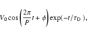
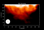
The prominence was located at high latitude, being part of a large polar-crown system, and showed significant time variations at several locations, although its global structure remained quite stable (compare Figs. 1a and 1b).

Figure 1: H$\beta$ image of the quiescent prominence a) at the beginning of the observational time sequence and b) at the end of the observational time sequence. The black band on the left of b) is caused by the slow drift of the image to the left during the observing time. The photosphere is located at the top of the image and the white line marks the edge of the prominence body. The letters A, B, C, D, E indicate the position of five points whose Doppler signal is shown in Fig. 2.

Open with DEXTER

Spectral images were flat-field corrected and median-filtered in order to eliminate intensity trends, dust specs and interference fringes across the field of view. Flat-field frames were obtained by drifting the telescope across the solar surface close to the Sun centre. In this way, solar features were averaged out. Further improvement was achieved by averaging several flat images.

During the observations and because of poor telescope tracking the image underwent a persistent drift towards the left which needed to be corrected before the data analysis could be carried out (see Movie 1). Superposed to this slow trend there was a very fast "jittering'' which was probably due to atmospheric image motion. This random jittering was arguably uncorrelated between the three wavelength images, since they were taken a few seconds apart, and did not introduce any neat displacement as time passed. Offsets in the x- and y-directions were calculated between consecutive images via a cross-correlation algorithm. This procedure was carried out independently for each wavelength position. Accumulated offsets for each wavelength display, in general, motions at two different time scales, which correspond to the long trend and fast image motions described above. Next, offsets were removed from the time series of images for each of the three wavelengths, which satisfactorily compensated for long trends and fast motions in the data sets. However, there remained the difficulty of aligning the images for the three wavelengths because the high-frequency image motion, together with the fact that the images at different wavelengths were not recorded at the same instant, gave rise to a small spatial displacement between those images. An inspection of the offsets revealed the presence of time intervals for which the relative offset for the three wavelength positions did not change much, probably because of a transient improvement in the observational conditions. The corresponding images were taken as reference frames and the accumulated offsets were referred with respect to them.

The resulting offset-corrected data set (see Movie 2) shows a perfectly still prominence and no signs of the long-term trends and image jittering present in the original data. The offset-corrected data have been used to calculate the Doppler shift, line width and line centre of the H$\beta$ line profile for each spatial point. Since the H$\beta$ line profile can be well modeled by a Gaussian curve (see Stellmacher & Wiehr 1995 and Molowny-Horas et al. 1999), the logarithm of the intensity has been interpolated with a second-order polynomial. Finally, the Doppler signals have been obtained at each point in the field of view and then two-dimensional Doppler velocity maps have been constructed, allowing us to carry out a temporal as well as spatial analysis.

As an example, in Fig. 2 we have plotted the Doppler velocity signals at five selected positions in the field of view, four inside and one outside the prominence structure. At low heights (point A) the signal is noisy, perhaps because of the effect of light coming from the photosphere. At larger heights in the prominence body (points B, C and D) the signal is much less noisy. The signal amplitude at point C, which shows a quasi-stationary behaviour with a clear defined period and a temporally damped profile, has increased considerably up to 4 km s^-1. On the other hand, the amplitude of the signal at point D, approximately at the same height, is rather small, at least for the first half of the observational time. For points outside the prominence body (like point E) the signal becomes very noisy probably because it comes from faint prominence parts outside the bright main prominence body (cf. Stellmacher & Wiehr 2000). It can be appreciated that different profiles of Doppler velocity signals can be found at different spatial locations in the prominence and that in some cases the signals show a strong oscillatory character. On the contrary, no significant periodicity has been detected in the line intensity or in the line width.

  
3 Temporal analysis of Doppler signals

3.1 Periodogram

Figure 2: Doppler velocity signal at points marked A, B, C, D, E in Fig. 1a. These signals are representative of the various features found in the observations. Points A and B display some hint of oscillations, the signal in the second one being quieter than in the first one. Points C and D show a clear temporal wave decay and amplification, while point E presents a noisy signal characteristic of coronal points. Each small tick mark in the vertical axis corresponds to a Doppler velocity of 1 km s-1.

Open with DEXTER

In order to analyse the dominant periods of Doppler velocity oscillations we have computed the Lomb-Scargle periodogram of the signal at each point. This technique, which has already been applied to the analysis of prominence oscillations (Sütterlin et al. 1997), is preferred over standard Fourier analysis since it provides with higher frequency resolution (see Scargle 1982; Horne & Baliunas 1986 and Carbonell & Ballester 1991). Note that if the period of the signal is not close to one of the Fourier frequencies, as usually happens when the signal has long periods (and indeed this is our situation), then Fourier analysis fails to provide an accurate value for the dominant period. On the other hand, the Lomb-Scargle periodogram allows a higher number of sampled frequencies and in consequence to resolve better the power peaks. This can be appreciated in Fig. 3, which shows the Lomb-Scargle periodogram and Fourier power spectrum for two of the Doppler velocity signals displayed in Fig. 2. Note, for example, the difference between both methods in the determination of the frequency of the most significant power peak in Fig. 3b. In this particular example, the Fourier power spectrum gives a period of 58 min, whereas the Lomb-Scargle periodogram yields a more precise period of 71 min.

Figure 3: a) Power spectrum from the Lomb-Scargle periodogram (continuous line) and Fourier analysis (dotted line joining circles, which are located at Fourier frequencies) for point A in Fig. 2. Due to the presence of noise in the signal many peaks are present in the periodogram, but only the one around 0.2 mHz is significant. b) The same for point C in Fig. 2, which shows that the peak located around 0.236 mHz (71 min) is found to be around 0.285 mHz (58 min) with the usual Fourier analysis. In both plots, the Lomb-Scargle periodogram consists of 181 equally spaced frequencies and the 99% confidence level (assuming a background white noise process, see Horne & Baliunas 1986) is given by the horizontal dashed line.

Open with DEXTER

Next we have performed a global analysis of the periods in the prominence structure by computing the Lomb-Scargle periodogram of the Doppler velocity in each point. In Fig. 4 we have represented the spatial distribution of period and spectral power for the highest peak in the power spectrum of each point. From Fig. 4a we can see that instead of an arbitrary distribution of periods, there are large regions, for example at the prominence centre or close to its lower edge (around position x=80, y=50), with similar values and even with similar power (see Fig. 4b). The periods in this region are in the 70-80 min range, although other values can be found in smaller areas within the prominence body. Periods around 30-40 min are, for example, detected at lower heights (a spatial variation of the period length was also observed by Wiehr et al. 1989). This means that there is a strong coherence in the period of oscillation at different locations over medium size areas of the prominence structure and so, from the data analysed here, oscillations with large power do not appear to be linked to small scales of the prominence. Nevertheless, it is not possible to rule out the presence of prominence fibril oscillations in the prominence under study, because the spatial resolution of the data is certainly not even close to one arcsec.

A final comment on the detected periods is in place. We are here selecting only those with large power in the periodogram (Fig. 4b) and covering wide prominence regions (at least $10 \times 10$ arcsec, say), since they provide us with the best evidence for oscillations of the cold prominence plasma. On the other hand, periods without enough significance in the periodogram and/or affecting smaller areas are discarded.

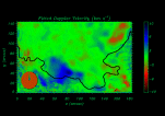
Figure 4: a) Spatial distribution of periods which correspond to the largest power peak in the periodogram and b) corresponding Lomb-Scargle spectral power values of the largest peak normalised to the overall maximum value. To make these figures, the power spectrum at each point in the field of view has been computed and the period and power of the largest peak in each periodogram have been kept. These two quantities have then been used to produce figures a) and b). The black and white line in the upper and lower panel, respectively, represents the prominence edge.

Open with DEXTER

3.2 Function fitting

Visual inspection of the signal at several positions in the prominence (see points C and D in Fig. 2 for some examples) suggests that in some cases the Doppler velocity can be described by an oscillating term which attenuates or amplifies in time (see also Molowny-Horas et al. 1999 and Terradas et al. 2001a). This particular behaviour of the Doppler signal can have strong physical implications and therefore any quantitative information about its damping time can provide valuable diagnostic information for, among others, the dissipation mechanism(s) acting in prominences. For this reason, the Doppler velocity at each point has been fitted by a function of the form

$$V_0\cos\left(\frac{2\pi}{P} t+\phi\right)\exp(-t/\mbox{${\tau}_{\rm D}$ }),$$ (1)

where V₀ is the amplitude, P is the period, $\phi$ is the phase and $\mbox{${\tau}_{\rm D}$ }$ is the damping time (for $\mbox{${\tau}_{\rm D}$ }>0$) or the growing factor (for $\mbox{${\tau}_{\rm D}$ }<0$). We have used this function to fit the Doppler velocity signal at each point in the field of view and have calculated the numerical values of the fitted parameters; examples of Doppler data and fitted values derived from Eq. (1) are given in Molowny-Horas et al. (1999) and Terradas et al. (2001a). Note that at some points in the prominence, Eq. (1) may not represent the observed signal, so in order to have a quantitative idea of the goodness of the fit we have computed the correlation coefficient, r, between the original signal and the fitted function. For those points in which the Doppler velocity is well represented by Eq. (1), the fitting of this function to the data allows us to improve the signal to noise level, while retaining the global behaviour of the signal.

	Figure 5: a) Fitted period for all the points in the field of view computed from Eq. (1). The continuous black line represents the approximate position of the edge of the prominence as seen in line centre. b) Correlation coefficient, r, between the original signal and the fitted function computed from Eq. (1) for all points in the prominence.
Open with DEXTER

To confirm the goodness of this ad hoc function we compare, for all points in the structure, the period obtained from a non-linear least-squares fit to Eq. (1) with the period that corresponds to the highest peak in the periodogram and shown in the previous subsection. A comparison between Figs. 4a and 5a reveals that the two methods yield a similar distribution of periods over the prominence body, with only minor discrepancies at a few small regions. This gives us more confidence on the fitted function as highly representative of the true signal. In particular, in the large region close to the edge of the prominence (around position x=80, y=50) the agreement is quite good. Moreover, in Fig. 5b we have plotted the computed correlation coefficient between the signal and Eq. (1) for all points. Note that there are large areas with correlation coefficients larger than 0.9 (for example in the region near the prominence edge mentioned before), while other points, such as those outside the prominence structure, have poor correlation coefficients. We can also compare the correlation coefficient with the power which corresponds to the largest peak in the periodogram normalised to its maximum value in the whole prominence (see Fig. 4b), which gives an idea of the strength of the periodicity. Again, there are large regions where the agreement is quite good, which provides with further evidence that the function given by Eq. (1) is in general a good representation of the Doppler velocity signal.

	Figure 6: a) Damping time computed from Eq. (1), with black colour representing growing velocity signals (i.e. $\mbox{${\tau}_{\rm D}$ }<0$) and white colour representing very long damping times ( $\mbox{${\tau}_{\rm D}$ }>500$ min), i.e. barely damped oscillations. b) Fitted amplitude, V0, computed from the same formula for all points in the prominence.
Open with DEXTER

We have next plotted $\mbox{${\tau}_{\rm D}$ }$ for all points (Fig. 6a) and again the most relevant feature is located near the prominence edge in the region where basically constant periods have been detected (around x=80, y=50). In this area the damping times display a practically uniform distribution with values approximately between two and three times the period (around 75 min), which represents a strong attenuation profile. On the other hand, although from Fig. 6a it seems that there are large regions for which the Doppler velocity amplifies in time, we have to point out that evolutionary changes at certain locations in the prominence structure may simulate quasi-oscillatory motions growing in time (see Sütterlin et al. 1997). Moreover, in general the correlation coefficient is poor for the black regions in Fig. 6a, which means that although the amplitude of the signal increases in time it cannot be well fitted by a simple exponential term.

It is also of interest to analyse the distribution of the computed amplitude, V₀ (Fig. 6b). Note that the amplitude (which is approximately the value of the Doppler velocity at the begining of the observational time) takes in general higher values at points where the signal attenuates than at points where it increases with time. Large velocity amplitudes are found, for example, localised around the right edge close to x=160, y=100 and also in the centre of the prominence body, around x=105, y=70. But again the most interesting region is located near the top edge of the prominence and specially in a large area around x=80, y=40, where the amplitude takes its maximum values. The spatial distribution of amplitudes at this location has an interesting geometrical structure. Large amplitudes seem to be localised along a channel parallel to the prominence edge. The amplitudes are in some cases quite large, specially near the edge, where they are around 10 km s^-1, but the mean value is around 2 km s^-1.

  
4 Spatial analysis of Doppler signals

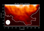
The presence of regions across which both the period and damping time display a certain degree of coherence is a clear indication that instead of arbitrary oscillations there are some kind of organised motions at these locations. In order to study these oscillatory motions we have also built movies showing the temporal evolution of the original Doppler velocity (Movie 3) and the fitted signal (Movie 4) for all points in the field of view. The movies show that close to the photosphere motions are of random type. On the contrary, although it is sometimes difficult to give a clear judgment on whether the observed periodicity represents steady oscillations or just some kind of internal activity of the prominence, there are several locations where periodic motions seem very clear. One of these regions is located close to the top edge of the prominence, where we have previously reported constant periods and where the signal has larger amplitudes. In Fig. 7 we display some frames of the Doppler velocity movie for different times. The presence of large amplitudes inside the region marked with a black rectangle can be clearly identified. In addition, positive and negative velocity patterns alternate in time (both in the centre of the rectangle and at its upper right corner) as it is specially noticeable in the first two frames. This phenomenon, which can be also found for other time steps and even in other regions, agrees well with the possible existence of a medium-size oscillatory pattern, as we have already pointed out. Moreover, with the help of the movie, propagating features can be also identified in this region, in particular close to the prominence edge. A detailed analysis of such traveling oscillatory motions can provide valuable information about plasma properties in that region through the computation of the phase speed and wavelength. We have concentrated our analysis on the region inside the rectangle in Fig. 7.

	Figure 7: Doppler velocity at times a) 20 min, b) 60 min and c) 100 min. The alternation of white (positive) and black (negative) velocities inside the black rectangle is a clear manifestation of an oscillatory phenomenon. The two particular paths marked in the last figure with continuous and dashed lines have been used to study the properties of waves in this area.
Open with DEXTER

4.1 Analysis of the signal along two selected paths

As a first step we have selected a particular path (continuous line in Fig. 7c) in the marked region and have plotted the Doppler velocity as a function of space (position along the path) and time, see Fig. 8a. It is interesting to compare this plot with that from the fitted Doppler velocity along the same path (Fig. 8b). The effect of the function fitting is quite clear: the global oscillatory behaviour is retained while small features have been smoothed out. The correlation coefficients along this path are in the range 0.85-0.98, which indicates that the fitted parameters have quite reliable values. Inspection of Fig. 8b reveals that some straight, bright and dark features are running across the image, indicating that a disturbance is traveling along the selected path. Moreover, one can see that these features possess constant slope, so that Figs. 8a and 8b are consistent with a plane propagating wave. The fact that the slope is negative for points roughly between 0 and 44, but positive for points between 44 and 62 indicates that propagation is to the left in the first case and to the right in the second case. The propagation speed along the path can be roughly calculated by measuring the slope of the bands in Fig. 8b. Computations give values around 15 km s^-1and 12 km s^-1 for propagation to the left and to the right, respectively, but these are just lower limits to the actual propagation speed since projection effects must be taken into account (Oliver & Ballester 2002). This comment applies to all the values of the phase speed and wavelength quoted in this paper. Note that, from the time interval between two consecutive white and dark features in Fig. 8b, the period of oscillation can be estimated to be around 75 min, in good agreement with Fig. 5a. In addition, the above values of propagation speed and period yield a tentative value of the wavelength (lower limit) along the selected path of 67 500 km and 54 000 km for propagation to the left and to the right, respectively.

	Figure 8: Plot of the Doppler velocity along a selected path (black line in Fig. 7c). a) Raw Doppler signal and b) fitted signal using Eq. (1). Bright and dark features, corresponding to positive and negative velocity amplitudes, propagate along the path both to the right (positions higher than 44) and to the left (positions lower than 44).
Open with DEXTER

A more exact determination of the wavelength and phase speed will be carried out next. The wavelength can be easily computed when several neighboring points are found to oscillate with basically the same period and when the signal is practically stationary, such as happens for the region under study. Under these circumstances, Fourier decomposition of the signal can provide useful information through the Fourier phase associated to the dominant period, computed at each of the spatial locations along the selected path. The presence of linear Fourier phase variations with distance is a clear indication of wave propagation, while an arbitrary spatial distribution of Fourier phases indicates non-organised oscillations (e.g. Molowny-Horas et al. 1997). Moreover, the derivative of the phase with position provides the wavelength. In Fig. 9 we have plotted the Fourier phase corresponding to the largest peak in the Fourier spectrum for each of the Doppler velocity signals represented in Fig. 8a. As we can see, there is an almost linear decrease of the phase between positions 5 and 30, a linear increase between positions 50 and 62 and a region of roughly constant phase in between. The first two patterns correspond to propagation to the left and right along the path, such as was pointed out from Fig. 8b, while the third pattern is caused by standing wave motions. The slope of straight lines fitted to the Fourier phase in each of the regions with wave propagation gives us the wavelength of oscillation, which is around 75 000 km and 70 000 km for the left and right propagating features, respectively. The corresponding phase velocities are around 17 km s^-1 and 15 km s^-1 for propagation to the left and to the right, respectively. These values are in good agreement with our previous, rough estimation.

Figure 9: Fourier phase associated to the largest peak in the Fourier spectrum vs. position along the black line in Fig. 7c. Propagation is towards the right at positions higher than 50 and towards the left for positions less than 30. The phase remains almost constant in the points with positions between 30 and 50, which indicates that there is some kind of wave generation at these points; the generated waves then propagate to both sides along this particular path.

Open with DEXTER

	Figure 10: a) Plot of the Doppler velocity for each position along the path shown in Fig. 7c as a dashed line. b) Plot of Fourier phase (corresponding to the dominant period) vs. position.
Open with DEXTER

As mentioned above, another interesting feature observed in the Doppler velocity movie is located close to the body centre (upper right corner in our small rectangle). We have represented the Doppler velocity as a function of space and time, see Fig. 10a, for the points along the dashed line in Fig. 7c. Now, at least for the first half of the observational time, positive and negative velocities seem to alternate in phase separated by a region, around position 25, with low amplitudes. This pattern suggests that rather than a propagating feature, the signal in this area behaves like a standing wave with two regions completely out of phase. During the second half of the observational time, some features seem to indicate propagation towards the right. Computation of the Fourier phase again gives a clear interpretation of the wave features (Fig. 10b). The Fourier phase is practically constant in a small region around position 10 and in a larger region for positions greater than 30, which indicates that the signal does not propagate in these locations. The phase difference between positions 10 and 50 is close to $\pi$, which, together with the fact that between these points the amplitudes take low values, is in close agreement with the standing wave picture and so a tentative identification of nodes and antinodes is possible. The estimated distance between the two antinodes visible in Fig. 10a is around 22 000 km, which implies that the wavelength of the standing wave is about 44 000 km and the corresponding phase speed is 10 km s^-1. These values are about half those previously obtained for propagation along the other selected path and are a consequence of the anisotropic propagation of the perturbation under study (see below).

4.2 Two-dimensional analysis of oscillations

The previous calculations, using the signal from points on a straight line, only provide a partial picture of the propagating or standing wave properties of the detected oscillations, just like what happens when one-dimensional observations using a fixed spectrograph slit are carried out. We have next obtained detailed information about the two-dimensional spatial variation of the wavelength and phase velocity inside the small rectangle in Fig. 7c. We start by plotting the Fourier phase for the most relevant period in the Fourier spectrum at each point (Fig. 11), which shows that a deep global minimum is found around the central position of the plot. This particular phase structure is an indication that motions have their origin at the position of the minimum and propagate, although in an anisotropic way, from this point. The noisy character of the signal outside the prominence gives rise to the irregular shape of the plot around the lower left corner of Fig. 11.

	Figure 11: Fourier phase associated to the largest peak in the Fourier spectrum for the particular region selected in Fig. 7c, both as a contour plot and as a surface plot. The selected paths plotted in Fig. 7c are also displayed with continuous and dashed straight lines. Note that cuts of the Fourier phase along these two paths give rise to Figs. 9 and 10b.
Open with DEXTER

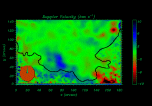
A much more clear interpretation of the two-dimensional phase can be gained from the wavevector field (Fig. 12). This magnitude is calculated as the gradient of the Fourier phase, being the natural extension of the phase derivative in the one dimensional case. The arrows indicate the direction of wave propagation, their length being proportional to the modulus of the wavenumber, k. The phase velocity field can be easily estimated from the usual formula, $v_{\rm ph}=\omega/k$, because waves in this particular region are basically monochromatic with period around 75 min. The phase velocity is also displayed in Fig. 12, where an upper bound around 30 km s^-1 has been selected to remove the values at phase minima (which have k=0 and so $v_{\rm ph}\rightarrow \infty$), that yield infinite phase velocity. The analysis of the wavevector field shown in Fig. 12 clearly indicates that motions seem to be generated in a narrow strip close to positions x=35-50 and y=30-20 and spread out from this region. It is remarkable, as mentioned before, that the direction of the propagating waves is basically parallel and towards the prominence edge from the source region, revealing the anisotropic character of the observed wave propagation. The values of the phase velocity are also quite different for both directions, being greater for the direction parallel to the edge, with $v_{\rm ph}\approx$20 km s^-1, than for the direction perpendicular to the edge, with $v_{\rm ph}\approx$ 10 km s^-1. This is an indication of the possible existence of some wave guiding phenomenon, which shows a preferential direction of propagation. Note the good agreement between the values of the phase velocity in the directions parallel and perpendicular to the edge and those derived from the analysis of the two selected paths.

It is worth noticing that small local minima in the Fourier phase must not be interpreted as other wave generation points because they are small irregularities in the global minimum shape. Note that these irregularities are specially relevant in points close to and outside the prominence edge.

Figure 12: Arrows represent the wavevector field computed from the gradient of the Fourier phase, displayed in Fig. 11, where the length of the arrows is proportional to the modulus of the wavevector. The phase velocity is shown with the help of different levels of grey and black and white colors. Strong gradients of the Fourier phase occur at the thin, dark band with almost zero phase velocity near the upper right corner. Therefore, large values of the wavevector are obtained and so the arrows in this band become so large that smaller arrows in the neighbourhood are difficult to appreciate. For this reason, such long arrows have been eliminated and dots have been plotted at the corresponding positions. The continuous black line depicts the position of the prominence edge.

Open with DEXTER

In order to analyse in more detail this anisotropic wave propagation, the Doppler velocity amplitude computed from the fit to Eq. (1), together with the wavevector field, are displayed in Fig. 13. It seems that higher amplitudes are localised in a region near the prominence edge, which, together with the wavevector distribution and with the phase velocity pattern, is indicative of the existence of some kind of wave guiding. Note also that the maximum of amplitude is not located at the point where waves seem to be generated, but is slightly shifted towards the edge. The direction of the arrows indicates that waves propagate from the source area to the region where the maximum amplitudes are detected.

On the other hand, from Fig. 13 we can see that the amplitude is quite small in the transition between the two regions (at the figure centre and upper right corner) oscillating $\pi$ rad out of phase, such as happens close to the nodes of a standing wave. In addition, the wavenumber takes large values at these locations, just as expected due to the sharp Fourier phase jump which results in the presence of strong gradients.

	Figure 13: Arrows represent the wavevector field computed from the phase gradient (see Fig. 12). The Doppler velocity amplitude fitted using Eq. (1) is shown with the help of different levels of grey and black and white colors. The continuous white line depicts the position of the prominence edge.
Open with DEXTER

	Figure 14: Arrows represent the wavevector field computed from the phase gradient (see Fig. 12). The damping times fitted using Eq. (1) are shown with the help of different levels of grey and white colour corresponds to regions where the signal amplitude increases in time, that is, it corresponds to growing times. The continuous black line shows the position of the prominence edge.
Open with DEXTER

Finally, in order to further expand the analysis of the source region, we have superimposed the damping times, computed from the fit to Eq. (1), to the wavevector field (see Fig. 14). We have restricted the plot to positive values of $\mbox{${\tau}_{\rm D}$ }$, which correspond to damped oscillations. Note that at locations of negative $\mbox{${\tau}_{\rm D}$ }$ (white areas), the amplitude and the correlation coefficient take small values, as can be appreciated by comparing with Figs. 5b and 13. The area shown in Fig. 14, as has been mentioned before, has damping times between two and three times the period, but only far away from the source region. On the other hand, close to the source region the distribution of damping times is really surprising, and of great interest from the physical point of view. The region where $\mbox{${\tau}_{\rm D}$ }$achieves its maximum values is located just over the wave generation area. This means that at the source region there is a practically constant contribution of energy while at the surrounding points, where energy has been propagated by the detected waves, an unknown damping mechanism exists which makes the Doppler velocity strongly attenuate in time. Unfortunately we do not have a clear explanation for this phenomenon.

  
5 Discussion and conclusions

In the present work we have analysed some wave propagation features associated to periodic Doppler shifts of a limb prominence. Using two-dimensional Doppler maps we have found some interesting properties that have not been reported before and that are of great physical interest. The most salient features are:

1.

The existence of large regions with periodic Doppler velocity oscillations with similar large periods around 75 min. This can be interpreted as a consequence of a global mode of oscillation of the prominence structure.

2.

By fitting a sinusoidal function multiplied by an exponential term to the observed Doppler velocity, the temporal damping of oscillations at several locations in the prominence has been characterised. The damping times are found to be between two and three times the period.

3.

The detailed analysis of a particular region with a specially strong velocity oscillation has allowed us to identify a wave generation profile associated with the global oscillatory pattern. Wave propagation along and across the prominence edge, with different phase velocity, has been also found, suggesting the action of a wave-guiding mechanism. The projected phase velocity has been calculated to be in the range 10-20 km s^-1.

The existence of similar periods over large areas (as big as 54 000 km $\times$ 40 000 km), which are often far away from one another, is in agreement with previous findings by Tsubaki et al. (1988) who found oscillations with the same period at two different heights in a quiescent prominence. Also, Balthasar et al. (1988) reported the presence of similar periods over the whole height of some prominences. On the other hand, the absence of small scale periodic variations can be related to the fact that our data lack the appropriate spatial resolution for the detection of very localised wave structures. This may be the reason why the observed oscillations excited medium size regions rather than smaller scale ones.

The most significant detected periods, around 70-80 min, fall in the long-period range. Similar values have been also reported by Bashkirtsev et al. (1983), Wiehr et al. (1984) and Bashkirtsev & Mashnich (1984). In particular, the last authors suggest that the 80 min periods are due to the chromospheric forcing, for which they have found the same value (see Mashnich & Bashkirtsev 1999). On the other hand, periods in the 30-40 min range are also observed in the prominence structure, although they are located in small regions. These periods have been also found by several authors, for example by Wiehr et al. (1984) and by Bashkirtsev & Mashnich (1984). On the contrary, we have not identified evidence in the power spectra of significant peaks in the short-period range. Possible reasons for the absence of this kind of oscillations in the data are that the corresponding MHD modes were not excited at the time observations were made or that they were excited but were associated to vertical plasma motions, which are hard to detect through the Doppler velocity in limb prominences.

Regarding the damping of oscillations, we have pointed out that they are a common feature in large areas, especially close to the edge of the prominence structure. Only minor documented evidence of such phenomenon exists in the literature, see for example Wiehr et al. (1989) and Tsubaki & Takeuchi (1986). In particular, the last authors reported Doppler fluctuations also near the edge of a prominence vaguely suggesting the presence of damped oscillations just at a few points. On the contrary, the attenuation behaviour found here affects a large area in the prominence and not just some points, which agrees with the possible presence of an energy dissipation mechanism that must be strong enough to produce the detected short damping times, typically between two and three times the period. Although the temporal decay profile found by Molowny-Horas et al. (1999), and used here to fit the Doppler velocity signal, is very well reproduced by an exponentially decreasing term, other physical processes acting in the prominence can have their own decay profile. Many mechanisms can be responsible for the damping of wave motions: optically thin or thick radiation, wave leakage, retardation effects due to the finite time required for perturbations to travel between the prominence and the photosphere (Schutgens 1997), etc. Moreover, Terradas et al. (2001b) have made an attempt to explain the possible exponential decay of perturbations in prominences by removing the usual adiabatic assumption in the energy equation in favour of Newton's cooling law. One of the conclusions of that work is that some combinations of low vertical wavenumbers and radiative relaxation times can give place to slow modes with long periods and short damping times, which is in good agreement with the results presented here. On the contrary, with the above mentioned energy dissipation mechanism, Alfvén and fast modes are not damped. Nevertheless, other physical effects can lead to the damping of these modes, e.g. damping of Alfvén waves by collisions between ions and neutral particles in the partially ionised prominence plasma (De Pontieu 1999; Pécseli & Engvold 2000).

As for negative values of the parameter $\tau_{\rm D}$, which could in principle be associated with signals increasing in time, they are usually found in points with small values of the correlation coefficient. Nevertheless, some locations with $\tau_{\rm D}<0$ display some hints of quasi-oscillatory motions growing in time (see Movies 2 and 3) that might be produced by evolutionary changes in the prominence plasma. The small values of the correlation coefficient obtained there, however, preclude us from being fully confident about this conclusion.

On the other hand, the detailed analysis of the oscillatory motions in a selected region has shown several interesting features. This analysis has allowed, with the help of the Fourier phase, to build, for the first time in prominences, a two-dimensional vector field showing the direction of wave propagation. We have found that travelling waves seem to be continuously generated in a narrow region which is located just over one of the antinodes of a pressumed standing wave. Travelling waves propagate anisotropically from the source region in the directions parallel and perpendicular to the prominence edge with different phase velocities. Such anisotropic propagation pattern can be a direct consequence of the particular plasma density profile in this channel parallel to the prominence edge, along which the density may be more or less uniform while showing a strong decrease when going from the prominence to corona across the channel. This mechanism is in good agreement with the spatial distribution of oscillatory amplitudes, which shows a clear increase from the region where waves are generated (x=45, y=25) to the region close to the prominence edge where waves propagate (x=40, y=15). However, it is difficult to draw a definitive interpretation because other effects, such as the magnetic field configuration or temperature distribution in the area or the projection along the line-of-sight, can lead to misleading conclusions.

Unfortunately we do not have information about the spatial distribution of physical variables in the prominence, which makes difficult to interpret the oscillations in terms of MHD waves. In addition, the exact geometry of this limb prominence is unknown, posing another inconvenient when trying to compare with theoretical models. Nevertheless, the value of the phase velocity, which is just a lower limit because of the effect of projection on the plane of the sky, has been calculated to be in the range 10-20 km s^-1 and agrees with the hypothesis of a slow (and thus compressional) wave rather than of Alfvénic nature. On the contrary, no intensity variations, which are usually associated with compression, have been detected. However, there is no clear evidence of correlation between Doppler velocity and line intensity or line width fluctuations in the literature of prominence oscillations.

To know the relationship between oscillations and the prominence structure in more detail and to give enough information for a theoretical interpretation, further observations are desirable. In particular, long observational times and acquisition of two-dimensional data are fundamental to determine the spatial arrangement of oscillatory parameters of interest, such as periods, propagation speeds, wavelengths, etc. Two-dimensional data series are also important to determine whether the existence of periodic perturbations is always associated with the fibril structure or not. On the other hand, the acquisition of two-dimensional data must be complemented with the use of adequate analysis tools, specially techniques designed to identify the dominant spatial and temporal structures in a data set which can then be linked to propagating/standing features that are associated with MHD waves (see Oliver & Ballester 2002 for further comments on possible observational experiments and techniques). We believe that the present kind of analysis is a potential powerful tool for the development of prominence seismology.

Acknowledgements

Eberhard Wiehr and Horst Balthasar are indebted to the German Science Foundation, DFG, for financial support. Eberhard Wiehr also acknowledges the kind support and hospitality of the staff members at the Sacramento Peak observatory. Jaume Terradas, Ramón Oliver and José Luis Ballester want to acknowledge the financial support received from MCyT under grant BFM2000-1329.

References

 
• Balthasar, H., Stellmacher, G., & Wiehr, E. 1988, A&A, 204, 286 In the text NASA ADS  
• Bashkirtsev, V. S., & Mashnich, G. P. 1984, Sol. Phys., 91, 93 In the text NASA ADS  
• Bashkirtsev, V. S., Kobanov, N. I., & Mashnich, G. P. 1983, Sol. Phys., 82, 443 In the text NASA ADS  
• Carbonell, M., & Ballester, J. L. 1991, A&A, 249, 295 In the text NASA ADS  
• De Pontieu, B. 1999, A&A, 347, 696 In the text NASA ADS  
• Engvold, O. 2001, in INTAS Workshop on MHD waves in Astrophysical Plasmas, ed. J. L. Ballester, & B. Roberts, 123, Universitat de les Illes Balears, Spain In the text  
• Horne, J. H., & Baliunas, S. L. 1986, ApJ, 302, 757 In the text NASA ADS  
• Mashnich, G. P., & Bashkirtsev, V. S. 1999, Sol. Phys., 185, 35 In the text NASA ADS  
• Molowny-Horas, R., Oliver, R., Ballester, J. L., & Baudin, F. 1997, Sol. Phys., 172, 181 In the text NASA ADS  
• Molowny-Horas, R., Wiehr, E., Balthasar, H., Oliver, R., & Ballester, J. L. 1999, in JOSO Annual Report '98, ed. A. Antalová, H. Balthasar, & A. Kucera (Astronomical Institute Tatranská Lomnica), p. 126 In the text  
• Pécseli, H., & Engvold, O. 2000, Sol. Phys., 194, 73 In the text NASA ADS  
• Oliver, R. 2000, in Magnetic Fields and Solar Processes, ed. A. Wilson, ESA SP-448, p. 425 In the text  
• Oliver, R. 2001, in INTAS Workshop on MHD waves in Astrophysical Plasmas, ed. J. L. Ballester, & B. Roberts, 133, Universitat de les Illes Balears, Spain In the text  
• Oliver, R., & Ballester, J. L. 2002, Sol. Phys., 206, 45 In the text NASA ADS  
• Scargle, J. D. 1982, ApJ, 263, 835 In the text NASA ADS  
• Schutgens, N. A. J. 1997, A&A, 325, 352 In the text NASA ADS  
• Stellmacher, G., & Wiehr, E. 1995, A&A, 299, 921 In the text NASA ADS  
• Stellmacher, G., & Wiehr, E. 2000, Sol. Phys., 196, 357 In the text NASA ADS  
• Sütterlin, P., Wiehr, E., Bianda, M., & Küveler, G. 1997, A&A, 321, 921 In the text NASA ADS  
• Terradas, J., Oliver, R., & Ballester, J. L. 2001a, in INTAS Workshop on MHD waves in Astrophysical Plasmas, ed. J. L. Ballester, & B. Roberts, 143, Universitat de les Illes Balears, Spain In the text  
• Terradas, J., Oliver, R., & Ballester, J. L. 2001b, A&A, 378, 635 In the text NASA ADS  
• Tsubaki, T. 1988, in Solar and Stellar Coronal Structures and Dynamics, ed. R. C. Altrock, 140 In the text  
• Tsubaki, T., & Takeuchi, A. 1986, Sol. Phys., 104, 313 In the text NASA ADS  
• Tsubaki, T., Toyoda, M., Suematsu, Y., & Gamboa, G. A. R. 1988, PASJ, 40, 121 NASA ADS  
• Vrsnak, B. 1993, Hvar Obs. Bull., 17, 23 In the text NASA ADS  
• Wiehr, E., Balthasar, H., & Stellmacher, G. 1984, Sol. Phys., 94, 285 In the text NASA ADS  
• Wiehr, E., Balthasar, H., & Stellmacher, G. 1989, Hvar Obs. Bull., 13, 131 In the text NASA ADS  
• Yi, Z., & Engvold, O. 1991, Sol. Phys., 134, 275 In the text NASA ADS  
• Yi, Z., Engvold, O., & Keil, S. L. 1991, Sol. Phys., 132, 63 NASA ADS

 

  
Online Material

 Movie 1

 Movie 2

 Movie 3

 Movie 4