Up: Local velocity field from galaxies
We consider the population of sosie galaxies for a calibrator of
absolute magnitude M0. The distribution function of its population Nis assumed to be Gaussian
 ;
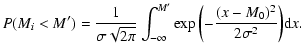
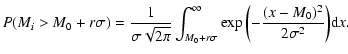
The probability for a galaxy of this population, to have an absolute magnitude Mi, with Mi<M' is given
by:
;
The probability for a galaxy of this population, to have an absolute magnitude Mi, with Mi<M' is given
by:
 |
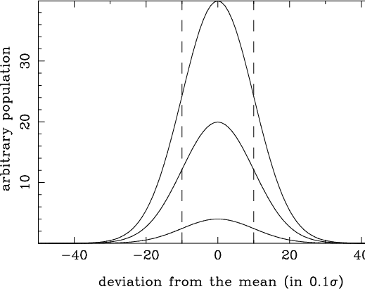
Figure A.1:
Several Gaussian functions with the same standard deviation  and different populations N. The actual range n x around the mean depends on
the population. and different populations N. The actual range n x around the mean depends on
the population. |
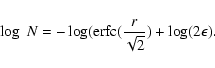
The difficulty is illustrated in Fig. A.1. With the same standard
deviation, the number of points beyond a given limit  increases
with the population N.
Our goal is to take into account this fact to
calculate the equation of the curve enveloping the points
of the Spaenhauer diagram.
increases
with the population N.
Our goal is to take into account this fact to
calculate the equation of the curve enveloping the points
of the Spaenhauer diagram.
Let us write the probability of having a galaxy with
 .
We will consider only this case but obviously, there is a similar case on the
other side of the Gaussian distribution.
.
We will consider only this case but obviously, there is a similar case on the
other side of the Gaussian distribution.
It is useful to take the centered variable u=x-M0:
 |
|
|
(A.1) |
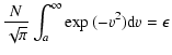
For a population of N observed galaxies, the probability for one of them to be at
from M0 is:
![$\displaystyle P\left(\bigcup_{i=1}^N{[M_{i}-M_{0} > r\sigma]}\right)$](/articles/aa/full/2002/37/aa9954/img236.gif) |
= |
 |
(A.2) |
because events are independent and have the same probability.
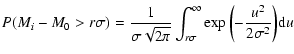
The criterion defining the upper limit of the points in the Spaenhauer
diagram is simply:
where  is an arbitrary probability level.
Then, using Eqs. (A.1) and (A.2), we obtain:
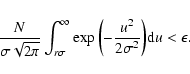 |
(A.3) |
With
 ,
the envelope equation becomes:
,
the envelope equation becomes:
where
 .
After integration, we obtain:
.
After integration, we obtain:
![\begin{displaymath}\frac{N}{2}\left[1-erf\left(\frac{r}{\sqrt{2}}\right)\right] = \epsilon
\end{displaymath}](/articles/aa/full/2002/37/aa9954/img244.gif) |
(A.4) |
i.e.,
 |
(A.5) |
 |
Figure A.2:
Representation of Eq. (A.5) for an arbitrary
probability level
 .
The curve (solid line) is the true
equation. The dashed line represents our linear representation for
a population between about 10 and 3000 galaxies. .
The curve (solid line) is the true
equation. The dashed line represents our linear representation for
a population between about 10 and 3000 galaxies. |
Figure A.2 shows the shape of the curve and the linear
representation we adopted over the population range 10 to 3000.
With
,
this linear representation is:
In fact, with a normalization procedure, we need only the slope which does
not depend on .
The number of galaxies observed up to a distance d is:
where  is the space density of the considered galaxies
and
is the space density of the considered galaxies
and  is the fractal dimension describing the distribution of
galaxies
(
is the fractal dimension describing the distribution of
galaxies
( in the case of homogeneous distribution).
Using the Hubble law (d=V/H), we obtain:
in the case of homogeneous distribution).
Using the Hubble law (d=V/H), we obtain:
Hence, the points of the envelop must fulfil simultaneously:
where b depends on
only and b' depends on ,
H.
The equation of the envelop obtained is then:
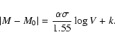 |
(A.6) |
The constant k depends on the values of ,
H.
We can find k (normalization) if we know a point of the curve.
This is done (see the main text) by imposing that the intersection of the
completeness curve with the envelope has an abscissa V0.05.
Up: Local velocity field from galaxies
Copyright ESO 2002
![$\displaystyle P\left(\bigcup_{i=1}^N{[M_{i}-M_{0} > r\sigma]}\right) < \epsilon$](/articles/aa/full/2002/37/aa9954/img238.gif)