A&A 393, 57-68 (2002)
DOI: 10.1051/0004-6361:20021018
J. N. Terry1 - G. Paturel1 - T. Ekholm 1
CRAL-Observatoire de Lyon, UMR 5574, 69230 Saint-Genis Laval, France
Received 24 May 2000 / Accepted 20 June 2002
Abstract
Pratton et al. (1997) showed that the velocity field around clusters
could generate an apparent distortion that appears as tangential structures
or radial filaments. In the present paper we determine the parameters of the
Peebles' model (1976) describing infall of galaxies onto clusters with the
aim of testing quantitatively the amplitude of this distortion.
The distances are determined from the concept of sosie galaxies (Paturel 1984) using 21 calibrators for which the distances were recently calculated from two independent Cepheid calibrations. We use both B and I-band magnitudes.
The Spaenhauer diagram method is used to correct for the Malmquist bias.
We give the equations for the construction of this diagram.
We analyze the apparent Hubble constant in different regions around Virgo
and obtain simultaneously the Local Group infall and the unperturbed Hubble
constant. We found:

We obtain the following mean distance moduli:
Key words: galaxies: general - galaxies: distances and redshifts - cosmology: distance scale - methods: statistical
The distribution of galaxies in the universe is seen as a foam with bubbles and voids.
This picture was predicted by Zel'dovich (1970) and
seen by Joeveer et al. (1978).
In the near universe these structures appear as large 2D filaments
or large 3D walls (de Lapparent et al. 1986; Haynes & Giovanelli 1986).
Indeed, the 3D distribution of galaxies built from their position and their radial
velocity clearly shows these kinds of structures. In Fig. 1
we plotted galaxies with known radial velocities in a slice of ![]() Mpc
around the plane defined by the closest superclusters
(Paturel et al. 1988). The polar direction, perpendicular to
this plane is about
Mpc
around the plane defined by the closest superclusters
(Paturel et al. 1988). The polar direction, perpendicular to
this plane is about
![]() and
and
![]() in galactic coordinates according to
Di Nella & Paturel (1994).
in galactic coordinates according to
Di Nella & Paturel (1994).
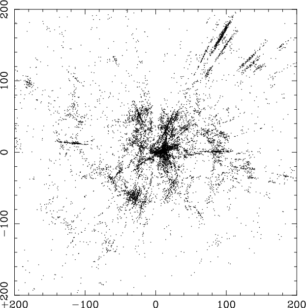 |
Figure 1:
Distribution of galaxies seen from their positions and radial velocities
within a slice of |
| Open with DEXTER | |
Pratton et al. (1997) showed that the velocity field around clusters could generate an apparent distortion which appears as tangential structures or radial filaments ("Finger of God''), similar to observed ones. A remarkable result shown by Rauzy et al. (1992) is that infall velocity does not affect the observed cosmological radial velocity for galaxies located on a sphere (hereafter the Rauzy sphere) having a diameter with ends at the position of the observer and at the center of the attractive galaxy cluster (on the Rauzy sphere, the infall direction is perpendicular to the line of sight). When plotting the distribution of galaxies with distances calculated from their observed radial velocities and a given Hubble constant (d=v/H), an artificial density enhancement on the Rauzy sphere is produced. This is illustrated in Fig. 2.
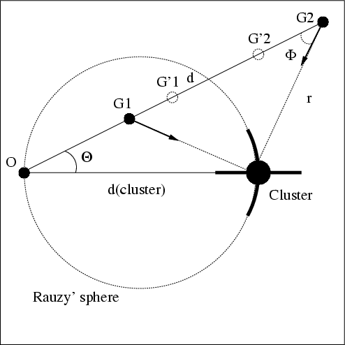 |
Figure 2:
Illustration of the apparent density enhancement around a
cluster.
A galaxy in position G1will be placed at position G'1 (because its radial velocity is
augmented by the projection |
| Open with DEXTER | |
This description, applied to near clusters, could lead to the scheme given in Fig. 3. This resembles the observed distribution of galaxies (Fig. 1).
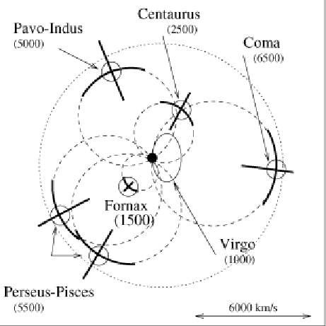 |
Figure 3: Illustration of the density enhancement around near clusters. The apparent density enhancement is shown for each cluster placed as in Fig. 1. Beyond the doted circle, the selection function on apparent magnitudes contributes to give the circular aspect (doted circle). The approximate mean radial velocity of each cluster is given in parenthesis under the name. |
| Open with DEXTER | |
A kinematical model is needed to give a more quantitative description.
The linearized model made by Peebles (1976) is a simple way to get
the infall velocities from a limited set of parameters. It leads to
the following equation of the infall velocity:
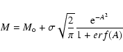
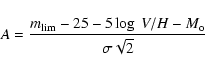
The spiral galaxies are good tracers of the velocity field because they are located, on average, in the outskirts of clusters. On the other hand, the relation between the absolute magnitude of a spiral galaxy and the rotation velocity of its disk (Tully & Fisher 1977) is the best known distance indicator. The method of sosie galaxies (look-alike galaxies) is a particular application of the Tully-Fisher method which bypasses some practical problems (Paturel 1984). However, the method does not correct for the Malmquist bias (Malmquist 1922; Sandage & Tammann 1975; Teerikorpi 1975) which has to be taken into account. The Spaenhauer diagram (Spaenhauer 1978; Sandage 1994) can be used to find galaxies not affected by this bias. In a recent paper (Paturel et al. 1998), the method of sosie galaxies and Spaenhauer diagram were presented for two calibrators (M 31 and M 81). The limited number of sosie galaxies didn't allow the present study. Here, we extend the method to 21 calibrators for which the distance has been recently calculated from the Cepheid Period-Luminosity relation using two independent zero-point calibrations. We use both B- and I-band magnitudes. The sample is deep enough to check directly Peebles' model.
In Sect. 2, we will select the calibrating galaxies and in Sect. 3 we will search for sosie galaxies of these selected calibrators. Then, in Sect. 4 we apply the Spaenhauer diagram method in order to select unbiased galaxies from which we analyze (Sect. 5) the Hubble constant in different regions around Virgo. In the direction of Virgo the comparison is made with predictions by Peebles' model.
The distance moduli of calibrators come from two independent calibrations of Cepheid Period-luminosity relations (Paturel et al. 2002a,b) based on the sample by Gieren et al. (1998) and on the HIPPARCOS Cepheid sample (Lanoix et al. 1999). The apparent magnitudes come from the LEDA database (http://www-obs.univ-lyon1.fr). They are corrected for galactic extinction and inclination effects following the precepts of Schlegel et al. (1998) and Bottinelli et al. (1995), respectively.
The Malmquist bias introduces a major difficulty in estimating
distances of astronomical objects.
It is caused to the fact that faint galaxies are missing in the sample
because of the limiting apparent magnitude (see the review paper by
Teerikorpi 1997).
To reach large distances with limited bias, we have to consider only
intrinsically bright galaxies.
Then, because the method of sosie galaxies selects galaxies having almost the same absolute
magnitude as calibrators, we have to consider the brightest calibrators.
On the other hand, we need a large sample and should not reject too many
calibrators.
The best compromise was judged from histograms of B- and I-absolute magnitudes.
We kept only calibrators satisfying either MB < -19 or MI < -21.
One calibrator (NGC 4603) was rejected because of the large uncertainty
on its distance modulus (0.86 mag).
The 21 remaining calibrators are presented in Table 1
as follows:
Column 1: PGC number from LEDA.
Column 2: NGC number.
Column 3: Distance modulus and its mean error (Paturel et al. 2002a,b).
Column 4: Morphological type from LEDA.
Column 5: Adopted inclination from LEDA following Fouqué et al. (1990).
Column 6: Internal extinction in B following Bottinelli et al. (1995).
Column 7: Galactic Extinction from Schlegel et al. (1998).
Column 8: ![]() ,
corrected B-magnitude from LEDA with its actual
uncertainty (Paturel et al. 1997).
,
corrected B-magnitude from LEDA with its actual
uncertainty (Paturel et al. 1997).
Column 9: Same as Col. 8 for I-band magnitudes. The corrections are 0.44 times
the B-band ones (Cols. 6 and 7). This 0.44 factor should be slightly
larger for the internal extinction (Han 1992) but for the method of sosie this correction vanishes
because the inclination is the same for the calibrator and its sosies.
Column 10: log of maximum rotation velocity and its actual uncertainty taken from LEDA.
It is calculated as a weighted mean of ![]() from both the 21-cm line width and
from both the 21-cm line width and
![]() rotation curve.
rotation curve.
| PGC | NGC | Type | i | Ai | Ag |
|
|||
| 0002557 | NGC 224 |
|
Sb | 78.0 | 0.67 | 0.46 |
|
|
|
| 0005818 | NGC 598 |
|
Sc | 55.0 | 0.38 | 0.18 |
|
|
|
| 0013179 | NGC 1365 |
|
SBb | 57.7 | 0.32 | 0.09 |
|
|
|
| 0013602 | NGC 1425 |
|
Sb | 69.5 | 0.54 | 0.06 |
|
|
|
| 0017819 | NGC 2090 |
|
Sc | 68.3 | 0.54 | 0.17 |
|
|
|
| 0028630 | NGC 3031 |
|
Sab | 59.0 | 0.38 | 0.35 |
|
|
|
| 0030197 | NGC 3198 |
|
SBc | 70.0 | 0.80 | 0.05 |
|
|
|
| 0031671 | NGC 3319 |
|
SBc | 59.1 | 0.48 | 0.06 |
|
|
|
| 0032007 | NGC 3351 |
|
SBb | 41.5 | 0.33 | 0.12 |
|
|
|
| 0032192 | NGC 3368 |
|
SBab | 54.7 | 0.21 | 0.11 |
|
|
|
| 0034554 | NGC 3621 |
|
SBcd | 65.6 | 0.64 | 0.35 |
|
|
|
| 0034695 | NGC 3627 |
|
SBb | 57.3 | 0.48 | 0.14 |
|
|
|
| 0039600 | NGC 4258 |
|
SBbc | 72.0 | 0.65 | 0.07 |
|
|
|
| 0040692 | NGC 4414 |
|
Sc | 54.0 | 0.41 | 0.08 |
|
|
|
| 0041471 | NGC 4496A |
|
SBd | 48.1 | 0.23 | 0.11 |
|
|
|
| 0041812 | NGC 4535 |
|
SBc | 44.0 | 0.20 | 0.08 |
|
|
|
| 0041823 | NGC 4536 |
|
SBbc | 58.9 | 0.62 | 0.08 |
|
|
|
| 0041934 | NGC 4548 |
|
SBb | 37.0 | 0.12 | 0.16 |
|
|
|
| 0042741 | NGC 4639 |
|
SBbc | 52.0 | 0.30 | 0.11 |
|
|
|
| 0043451 | NGC 4725 |
|
SBab | 54.4 | 0.23 | 0.05 |
|
|
|
| 0069327 | NGC 7331 |
|
Sbc | 75.0 | 0.62 | 0.39 |
|
|
|
The use of some calibrators (e.g., NGC 598 and NGC 4496A) is debatable because they are faint with poor photometry. This point is discussed in Sect. 5.
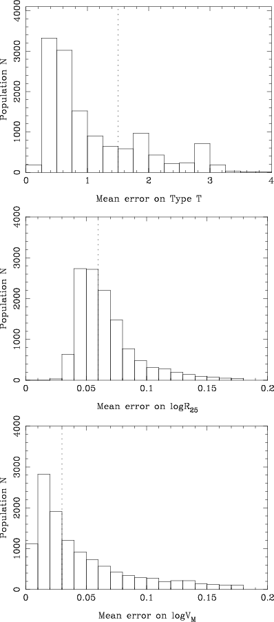 |
Figure 4:
Histogram of actual uncertainties on morphological type code T,
log of axis ratio
|
| Open with DEXTER | |
Thus, we define a sosie of a calibrator
with the following conditions (the parameters of the calibrator are noted with
the upperscript "calib''):
| (2) |
 |
(3) |
 |
(4) |
The application of the previous criteria to galaxies of the
LEDA2002 gives a sample of 2732 galaxies which are sosie of one of the 21
calibrators of Table 1.
495 galaxies are sosie of two or three
calibrators![]() .
For these galaxies we compared the distance moduli obtained from
different calibrators.
The mean standard deviation of their distance moduli is 0.29.
.
For these galaxies we compared the distance moduli obtained from
different calibrators.
The mean standard deviation of their distance moduli is 0.29.
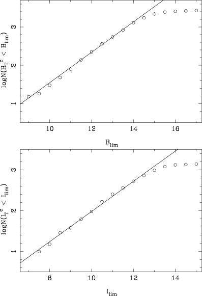 |
Figure 5:
Completeness curve for the B and I-band apparent magnitudes. The
curve begins to bend down at |
| Open with DEXTER | |
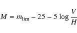
The limiting apparent magnitude is
![]() mag in B and
mag in B and
![]() mag in I.
The slopes are
mag in I.
The slopes are
![]() and
and
![]() ,
for B and I respectively.
The result that the slope is smaller than the theoretical one has already been
discussed (Paturel et al. 1994; Teerikorpi et al. 1998).
In the following sections we will use the observed slope (0.4) and the limits
14 and 12.5 for B and I magnitudes.
,
for B and I respectively.
The result that the slope is smaller than the theoretical one has already been
discussed (Paturel et al. 1994; Teerikorpi et al. 1998).
In the following sections we will use the observed slope (0.4) and the limits
14 and 12.5 for B and I magnitudes.
The construction of the Spaenhauer diagram requires three curves:
 |
(6) |
 |
(7) |
 |
(8) |
 |
(9) |
 |
(10) |
 |
(11) |
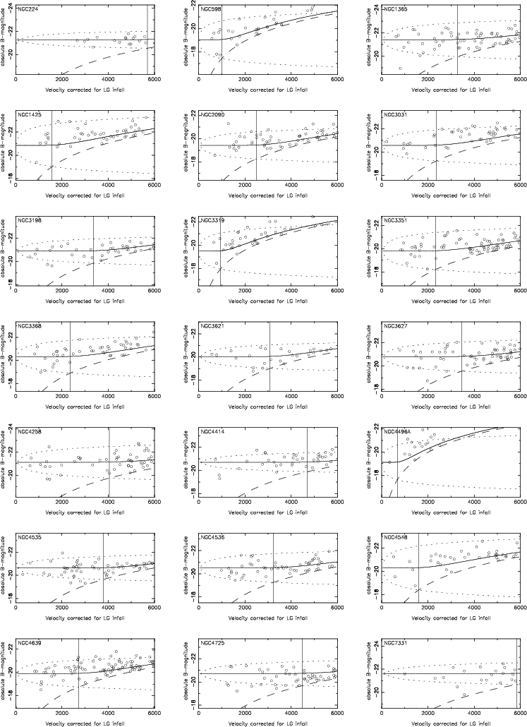 |
Figure 6: Spaenhauer diagrams in B magnitudes. For each calibrator we plot its sosie galaxies, with the predicted envelope (doted curve). The bias curve is show as a solid curve. The region of completeness is above the dashed curve. Finally, the unbiased region ("plateau'') is defined on the left of the vertical line. The name of the calibrating galaxy is indicated in the upperleft corner of each frame. |
| Open with DEXTER | |
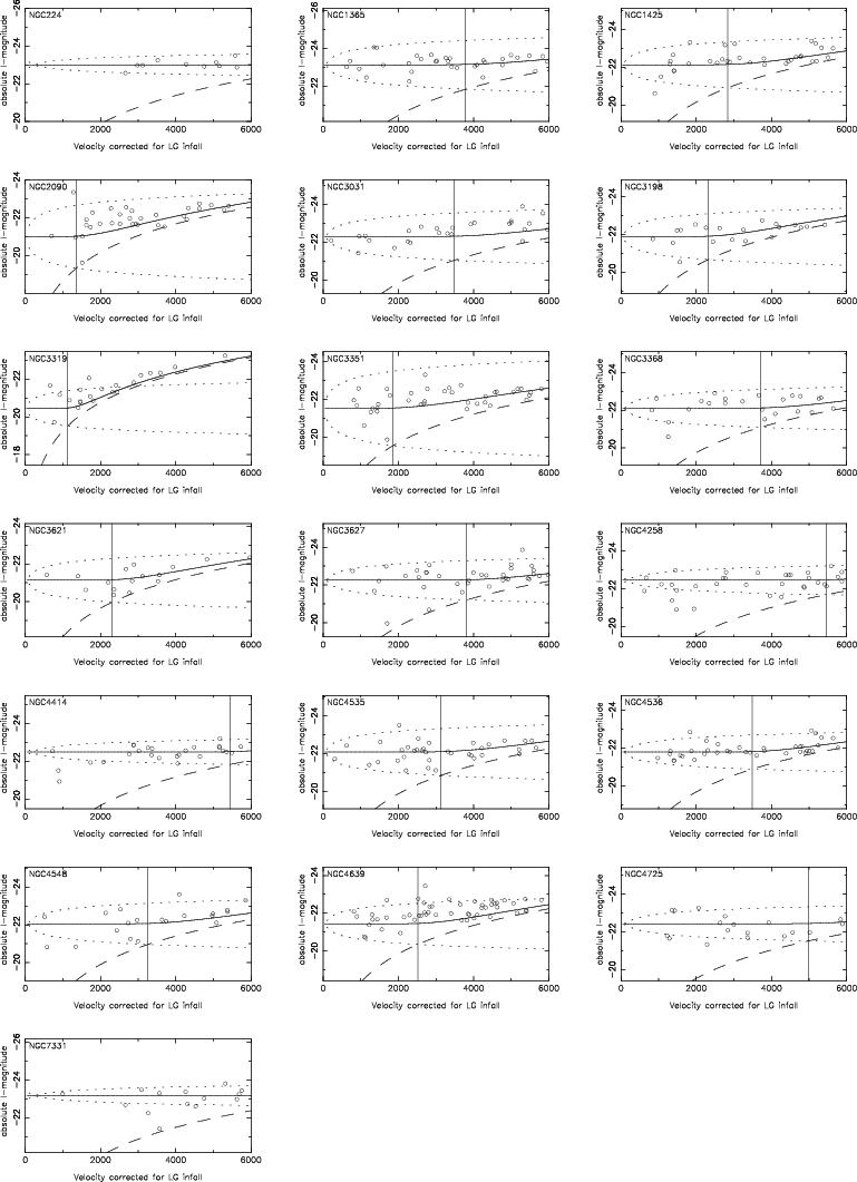 |
Figure 7: Spaenhauer diagrams in I magnitudes (same as Fig. 6). |
| Open with DEXTER | |
 |
(12) |
 |
(13) |
 |
(14) |
The mean error on the mean distance modulus is then:
 |
(15) |
| PGC | Alternate name | RA.DEC.2000 |
|
||
|
|
km s-1 | ||||
0004596 |
NGC 452 | J011614.8+310201 | 5078 |
|
135.2 |
| 0005035 | NGC 494 | J012255.4+331025 | 5582 |
|
132.8 |
| 0005268 | NGC 523 | J012520.8+340130 | 4881 |
|
131.8 |
| 0010048 | NGC 1024 | J023911.8+105049 | 3522 |
|
140.6 |
| 0014906 | NGC 1558 | J042016.1-450154 | 4278 |
|
121.6 |
| 0016359 | UGC 3207 | J045609.8+020926 | 4494 |
|
112.6 |
| 0018739 | UGC 3420 | J061601.8+755611 | 5353 |
|
78.9 |
| 0021336 | NGC 2410 | J073502.5+324921 | 4769 |
|
69.9 |
| 0026101 | IC530 | J091517.0+115309 | 4981 |
|
47.7 |
| ... |
We can now start the study of the local velocity field around Virgo from this unbiased sample.
The histograms of ![]() derived from B and I are presented in Fig. 8. The visible result is that both photometric bands give the
same mean.
derived from B and I are presented in Fig. 8. The visible result is that both photometric bands give the
same mean.
The means
![]() and
and
![]() are obviously not significantly different from each other.
This justifies that the distance moduli in B and I are combined as explained in
the previous section.
Similarly, the
are obviously not significantly different from each other.
This justifies that the distance moduli in B and I are combined as explained in
the previous section.
Similarly, the ![]() will be now the weighted mean of
will be now the weighted mean of ![]() in B and I.
In order to see the influence of Virgo, we plot now
in B and I.
In order to see the influence of Virgo, we plot now ![]() vs.
vs. ![]() .
Three regions are defined (Fig. 9):
.
Three regions are defined (Fig. 9):
Let us study in detail these regions with the target of fitting Peebles' model.
In region III the influence of Virgo is small on individual galaxies because they
are far from the Virgo center but the infall of our Local Group may be not
negligible. If the adopted LG-infall is too large the ![]() for this region
will be too high (and vice versa).
On the contrary, in region Ib (i.e., region I without the central region Ia of
the Virgo center)
one expects
for this region
will be too high (and vice versa).
On the contrary, in region Ib (i.e., region I without the central region Ia of
the Virgo center)
one expects ![]() to diminish when the adopted LG-infall increases. This
is confirmed by Fig. 10 where we calculated the mean
to diminish when the adopted LG-infall increases. This
is confirmed by Fig. 10 where we calculated the mean ![]() in regions Ib and III for different LG-infall velocities. The error bar on
each point is used to define internal uncertainties on
in regions Ib and III for different LG-infall velocities. The error bar on
each point is used to define internal uncertainties on
![]() and
and
![]() .
.
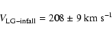
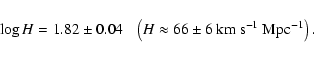
The intersection of the two curves of Fig. 10 gives accurately
both the infall velocity of the LG and ![]() .
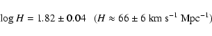
We obtain:
.
We obtain:
 |
(16) |
 |
(17) |
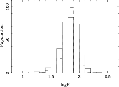 |
Figure 8:
Histograms of |
| Open with DEXTER | |
 |
Figure 9:
Mean |
| Open with DEXTER | |
| |
Figure 10:
Determination of the LG infall velocity onto Virgo and of
the corrected Hubble constant. The full curve represents how |
| Open with DEXTER | |
In order to search for possible residual bias, we plotted the mean ![]() of each
calibrator class versus the absolute magnitude of its calibrator, in Band I-band, (Fig. 11).
A tendency to have large
of each
calibrator class versus the absolute magnitude of its calibrator, in Band I-band, (Fig. 11).
A tendency to have large ![]() when the calibrator is
faint might be present for the less luminous calibrator. The slope of this
relation is
when the calibrator is
faint might be present for the less luminous calibrator. The slope of this
relation is
![]() .
This is barely significant at the 0.01 probability level
(to be significant, the Student's t test requires
t0.01>2.57, while we observe
t=0.015/0.006=2.5). If one removes the six less luminous calibrators
(NGC 598, NGC 4496A, NGC 2090, NGC 3319, NGC 3351 and NGC 4639), the
tendency disappears (t=0.4). In this case, the mean log of the Hubble constant
becomes
.
This is barely significant at the 0.01 probability level
(to be significant, the Student's t test requires
t0.01>2.57, while we observe
t=0.015/0.006=2.5). If one removes the six less luminous calibrators
(NGC 598, NGC 4496A, NGC 2090, NGC 3319, NGC 3351 and NGC 4639), the
tendency disappears (t=0.4). In this case, the mean log of the Hubble constant
becomes
![]() (instead of
(instead of
![]() ). Thus, the mean
Hubble constant is not severely affected, but small
). Thus, the mean
Hubble constant is not severely affected, but small
![]() is probably better.
is probably better.
| |
Figure 11:
Relation between the mean |
| Open with DEXTER | |
 |
(18) |
 |
(19) |
Now, we can plot
![]() vs. r (Fig. 12) to check directly
Peebles' model (Eq. (1)).
From the previous relation it can be seen that the errors on
x- and y-axis are strongly correlated.
The dominant error comes from d.
The asymptotic velocity infall is zero at large r distances. The location of the LG is
represented by a large open square.
We calculated
vs. r (Fig. 12) to check directly
Peebles' model (Eq. (1)).
From the previous relation it can be seen that the errors on
x- and y-axis are strongly correlated.
The dominant error comes from d.
The asymptotic velocity infall is zero at large r distances. The location of the LG is
represented by a large open square.
We calculated ![]() by minimizing the dispersion on
by minimizing the dispersion on
![]() .
For this
calculation we limited r between 3 Mpc and 30 Mpc in order to avoid the Virgo
center, where there is a very large uncertainty on
.
For this
calculation we limited r between 3 Mpc and 30 Mpc in order to avoid the Virgo
center, where there is a very large uncertainty on
![]() due to the small
value of r.
The best result is obtained for
due to the small
value of r.
The best result is obtained for
![]() .
This result is quite comparable with the value
adopted by Peeblees (
.
This result is quite comparable with the value
adopted by Peeblees (![]() )
but the uncertainty, estimated visually, is large
(about 0.2). The application to the Local Group infall leads to
)
but the uncertainty, estimated visually, is large
(about 0.2). The application to the Local Group infall leads to
![]() .
In order to highlight the tendency, we plot the mean x and y values of individual points
in four x-boxes: (3 to 7) Mpc, (7 to 13) Mpc, (13 to 21) Mpc and (21 to 31) Mpc.
These mean points (open circles) are represented with their observed scatter divided by
the square root of the number of points in each box.
.
In order to highlight the tendency, we plot the mean x and y values of individual points
in four x-boxes: (3 to 7) Mpc, (7 to 13) Mpc, (13 to 21) Mpc and (21 to 31) Mpc.
These mean points (open circles) are represented with their observed scatter divided by
the square root of the number of points in each box.
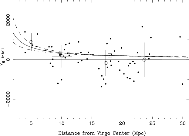 |
Figure 12:
Direct determination of the parameters of Peebles' model.
The adopted model is represented with the solid curve. Dashed curves
correspond to a change of |
| Open with DEXTER | |
It is interesting to see in detail which galaxies are exactly in the direction of
the Virgo center. If we consider galaxies with
![]() and
and
![]() only 9 galaxies remain. They are presented in Table 3 following increasing
radial velocities. For each galaxy we give the observed Hubble constant H.
In this table two parameters are independent: the radial velocity and the distance
modulus.
only 9 galaxies remain. They are presented in Table 3 following increasing
radial velocities. For each galaxy we give the observed Hubble constant H.
In this table two parameters are independent: the radial velocity and the distance
modulus.
| PGC | NGC |
|
H | ||
| 0041934 | NGC 4548 | 587 |
|
2.4 | 38 |
| 0042833 | 917 |
|
5.1 | 39 | |
| 0043798 | 1089 |
|
11.7 | 38 | |
| 0042741 | NGC 4639 | 1097 |
|
3.1 | 50 |
| 0043451 | NGC 4725 | 1360 |
|
13.9 | 94 |
| 0041823 | NGC 4536 | 1846 |
|
10.2 | 120 |
| 0041812 | NGC 4535 | 2029 |
|
4.3 | 129 |
| 0041024 | 2069 |
|
4.7 | 114 | |
| 0042069 | 2342 |
|
1.8 | 119 | |
| Mean |
|
||||
| Adopted |
|
The main feature from this table is that the apparent Hubble constants are
sorted according to velocities. This means that the distance does not
intervene very much. The natural interpretation is that all these galaxies
are almost at the same distance (distance of Virgo). The Hubble constant
reflects only the infall velocity.
Large velocities correspond
to galaxies in front of Virgo and falling onto Virgo, away from us. On the contrary,
galaxies with small velocities are beyond Virgo and falling onto it in our direction.
Indeed, the four galaxies with small velocities have a mean distance modulus
of
![]() while the four galaxies with high velocities have a larger
mean distance modulus of
while the four galaxies with high velocities have a larger
mean distance modulus of
![]() .
The difference is significant at
about
.
The difference is significant at
about ![]() .
This confirms clearly the interpretation.
From the table one can conclude that the distance modulus of Virgo is
.
This confirms clearly the interpretation.
From the table one can conclude that the distance modulus of Virgo is
![]() .
However, it is difficult to give a mean radial velocity
because of the strong perturbation of the velocity field. Amazingly, it
is better to measure radial velocities out of the center to obtain a good
mean velocity of a cluster. If one adopts the velocity
of 980 km s-1 (see the discussion in Teerikorpi et al. 1992),
and both the LG-infall velocity and the Hubble constant
found in this paper, the distance modulus of the Virgo cluster is
.
However, it is difficult to give a mean radial velocity
because of the strong perturbation of the velocity field. Amazingly, it
is better to measure radial velocities out of the center to obtain a good
mean velocity of a cluster. If one adopts the velocity
of 980 km s-1 (see the discussion in Teerikorpi et al. 1992),
and both the LG-infall velocity and the Hubble constant
found in this paper, the distance modulus of the Virgo cluster is ![]() .
This gives a coherent system of parameters.
.
This gives a coherent system of parameters.
We can also discuss the region perpendicular to the direction of Virgo
(region II). The weighted mean Hubble constant in this region is
nearly the same as the one found in region III (i.e.,
![]() ).
In the direction of the Fornax cluster one can repeat what we have done
in the direction of Virgo, but the number of galaxies is smaller.
The center of Fornax is assumed to be
).
In the direction of the Fornax cluster one can repeat what we have done
in the direction of Virgo, but the number of galaxies is smaller.
The center of Fornax is assumed to be
![]() and
and
![]() .
In Table 4 we summarize the results. It appear that
galaxies PGC 12390 and PGC 10330 can be considered as backside galaxies
falling onto Fornax
towards us (small radial velocity, large distance, small apparent
Hubble constant). Galaxies PGC 13255 and PGC 13602 are roughly at the
position of Fornax, while PGC13179 and PGC 13059 are in front of Fornax
(large radial velocity, small distance and large apparent Hubble constant).
From the table one can conclude that the distance modulus of Fornax is
.
In Table 4 we summarize the results. It appear that
galaxies PGC 12390 and PGC 10330 can be considered as backside galaxies
falling onto Fornax
towards us (small radial velocity, large distance, small apparent
Hubble constant). Galaxies PGC 13255 and PGC 13602 are roughly at the
position of Fornax, while PGC13179 and PGC 13059 are in front of Fornax
(large radial velocity, small distance and large apparent Hubble constant).
From the table one can conclude that the distance modulus of Fornax is
![]() .
It is not possible to measure how the infall velocity changes with the distance
to the center of Fornax. Nevertheless, if one still adopt
.
It is not possible to measure how the infall velocity changes with the distance
to the center of Fornax. Nevertheless, if one still adopt
![]() one can determine the parameter C for Fornax. Indeed, the observed infall velocity
is roughly 270 km s-1 at a distance of 6 Mpc of the center.
This leads to
one can determine the parameter C for Fornax. Indeed, the observed infall velocity
is roughly 270 km s-1 at a distance of 6 Mpc of the center.
This leads to
![]() .
.
| PGC |
|
H | ||
| 0012390 | 767 |
|
14.5 | 31 |
| 0010330 | 1249 |
|
14.4 | 36 |
| 0013255 | 1279 |
|
11.1 | 53 |
| 0013602 | 1299 |
|
6.0 | 65 |
| 0013179 | 1423 |
|
2.1 | 91 |
| 0013059 | 1670 |
|
3.4 | 91 |
| Mean |
|

The next step will be an application of this model to nearby clusters. The purpose is to test quantitatively the amplitude of the distortion on the apparent galaxy distribution induced by infalls.
Acknowledgements
We thank the anonymous referee and P. Fouqué for their remarks. T.E. acknowledges the support by the Academy of Finland (the projects "Galaxy Streams and Structures in the nearby Universe'' and "Cosmology in the local to the deep galaxy universe'').
 |
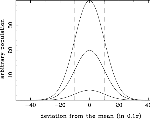 |
Figure A.1:
Several Gaussian functions with the same standard deviation |
The difficulty is illustrated in Fig. A.1. With the same standard
deviation, the number of points beyond a given limit ![]() increases
with the population N.
Our goal is to take into account this fact to
calculate the equation of the curve enveloping the points
of the Spaenhauer diagram.
increases
with the population N.
Our goal is to take into account this fact to
calculate the equation of the curve enveloping the points
of the Spaenhauer diagram.
Let us write the probability of having a galaxy with
![]() .
We will consider only this case but obviously, there is a similar case on the
other side of the Gaussian distribution.
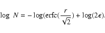
.
We will consider only this case but obviously, there is a similar case on the
other side of the Gaussian distribution.
 |
The criterion defining the upper limit of the points in the Spaenhauer
diagram is simply:
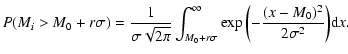
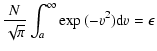
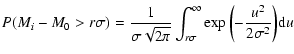
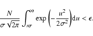
![$\displaystyle P\left(\bigcup_{i=1}^N{[M_{i}-M_{0} > r\sigma]}\right) < \epsilon$](/articles/aa/full/2002/37/aa9954/img238.gif) |
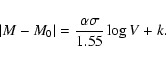
Then, using Eqs. (A.1) and (A.2), we obtain:
 |
| |
Figure A.2:
Representation of Eq. (A.5) for an arbitrary
probability level
|
Figure A.2 shows the shape of the curve and the linear
representation we adopted over the population range 10 to 3000.
With
![]() ,
this linear representation is:
,
this linear representation is:
The equation of the envelop obtained is then:

![$\displaystyle P\left(\bigcup_{i=1}^N{[M_{i}-M_{0} > r\sigma]}\right)$](/articles/aa/full/2002/37/aa9954/img236.gif)
![\begin{displaymath}\frac{N}{2}\left[1-erf\left(\frac{r}{\sqrt{2}}\right)\right] = \epsilon
\end{displaymath}](/articles/aa/full/2002/37/aa9954/img244.gif)