3 X-ray data and analysis

The X-ray observing logs for both clusters are given in Table 7. For both ROSAT/HRI images we have used $5\hbox{$^{\prime\prime}$ }$/pixel binning of the event list in order to reduce the noise as much as possible without losing information on the cluster extension. The raw photon images were then filtered using wavelet analysis with Poisson noise modeling (Starck & Pierre 1998) at 10^-4 ($\sim$$4\sigma$) significance level for the wavelet coefficients.

 

 

Table 2: Summary of the multi-slit spectroscopic observations.

Date	Object	RA Dec	Airmass	MOS	Exposure
		(J2000)		masks/slits	(s)
1993 Mar. 29	Abell 1451	12:03:15 -21:31:36	1.2	1/15	900
1993 Mar. 29	RXJ1314-25	13:14:29 -25:16:25	1.1	1/15	2$\times$900+1800
1999 Apr. 19/20	Abell 1451E	12:03:12 -21:33:25	1.34	2/20+21	3$\times$1800/4$\times$2100
1999 Apr. 19/20	Abell 1451W	12:03:23 -21:33:25	1.40	2/21+19	2$\times$3600/4200
1999 Apr. 19/20	RXJ1314-25N	13:14:22 -25:14:55	1.06	2/17+18	2$\times$3600/4$\times$2100
1999 Apr. 19/20	RXJ1314-25S	13:14:22 -25:17:55	1.04	2/17+18	4$\times$1800/4$\times$2100

Figure 3: RXJ1314-25: I-band image from the Danish 1.5-m telescope showing the objects in the spectroscopic study. Numbers correspond to the object identifications in Table 4; those marked with diamonds denote either stars or non-cluster members. Note that we have not plotted galaxy #20 because it is not resolved spatially from galaxy #19.

3.1 X-ray morphology

The X-ray contours are shown overlaid on optical images and radio observations (see Sect. 4) in Fig. 7 for Abell 1451 and in Fig. 8 for RXJ1314-25.

 

 

Table 5: Abell 1451: some statistical characteristics of the redshift distribution, corrected for measurement errors (Danese et al. 1980). The scale measure is in the cluster rest frame, i.e., $S_{{\rm BI}} = c\sigma _z/(1+z)$ (Harrison 1974). The errors ($1\sigma$) are calculated by using the accelerated bias-corrected bootstrap technique with 1000 bootstrap resamplings (Efron & Tibshirani 1986).

Characteristic	Value
N = 57
Bi-weighted location: $C_{{\rm BI}}$	$\overline{z}=0.1989^{+0.0005}_{-0.0007}$
Bi-weighted scale: $S_{{\rm BI}}$	1330+130-90 km s-1
Maximum gap	564 km s-1

3.1.1 Abell 1451

The X-ray image in Fig. 7 shows a very strong point source $\sim$ $1\hbox{$^\prime$ }30\hbox{$^{\prime\prime}$ }$ south of the cluster centre which coincides with a QSO at z=1.17 (object #32 in Table 3). The cluster emission is regular, with the inner contours slightly twisted but no sign of substructure. The X-ray emission peaks at RA = $12^{\rm h}03^{\rm m}16\hbox{$.\!\!^{\rm s}$ }6$ and Dec = $-21\hbox{$^\circ$ }32\hbox{$^\prime$ }21\hbox{$^{\prime\prime}$ }$, which is $36\hbox{$^{\prime\prime}$ }$ (150 kpc) north of the brightest cluster galaxy (#34 in Table 3) and $12\hbox{$^{\prime\prime}$ }$ west of the second brightest galaxy (#39), and $\sim$ $1\hbox{$^\prime$ }40\hbox{$^{\prime\prime}$ }$ from the catalogued cluster position (Abell et al. 1989).

3.1.2 RXJ1314-25

The cluster X-ray emission is quite irregular, showing two central peaks and a SE-NW elongation. Unfortunately, there is an X-ray emitting star projected in front of the cluster (object #29 in Table 4) only $\sim$ $24\hbox{$^{\prime\prime}$ }$ from the adopted X-ray centre. The strong point source SE of the cluster centre is a Sy1 galaxy (object #47 in Table 4) and a cluster member. There is no indication of substructure in the X-ray emission associated with the eastern group or the brightest cluster galaxy (see Fig. 6).

3.2 X-ray properties

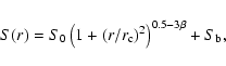
To estimate the basic physical cluster parameters we model the X-ray surface brightness using the isothermal $\beta$-model (King 1962; Cavaliere & Fusco-Femiano 1976)

$$% S(r) = S_0\left(1 + (r/r_{\rm c})^2\right)^{0.5 - 3\beta} + S_{\rm b},$$ (1)

where S(r) is the azimuthally averaged X-ray surface brightness as a function of the radial distance r from the centre, S₀ is the central brightness, $S_{\rm b}$ is the background contribution and $r_{\rm c}$ is the core radius. To fit the model profile to the data we define a proper cluster centre and exclude any discrete sources projected over the cluster X-ray emission. Finally, we obtain an average profile by summing the cluster X-ray photons in concentric rings and fit the model (Eq. (1)) with $S_0,\ S_{\rm b},\ \beta$ and $r_{\rm c}$ as free parameters, taking into account the Poissonian errors of the rings counts. The X-ray surface brightness profiles of Abell 1451 and RXJ1314-25 are shown in Figs. 9, 10, with the corresponding parameters in Table 8.

To derive the count-rate in the [0.1-2.4] keV ROSAT/HRI band we integrate the fitted surface brightness profile analytically, excluding the background. The integration is usually carried out to a given radius $r_{\rm lim}$, where the surface brightness profile reaches the detection limit; for both clusters we put $r_{\rm lim}=300\hbox{$^{\prime\prime}$ }$. For the overall count rate C we have

 

$$% C(<r_{\rm lim}) = \int_{0}^{r_{\rm lim}} 2\pi r S(r){\rm d}r = ... ...t[\left (1+\left(r_{\rm lim}/r_{\rm c}\right)^2\right)^{3/2-3\beta} - 1\right].$$ (2)

By means of EXSAS (Zimmermann et al. 1994), the observed count-rate is then used to normalize the spectral model - a Raymond & Smith (1977) thermal plasma emission, convolved by the ROSAT/HRI response function, with temperature and metallicity from ASCA data (Matsumoto et al. 2001) and line-of-sight Galactic absorption by H I from Dickey & Lockman (1990). The spectrum is then integrated to derive the flux and cluster rest frame luminosity in the "standard'' X-ray bands [0.5-2] and [2-10] keV. The profile model, together with the emission model, was used to derive the emission measure, $\int_{V} n_{\rm e} n_{\rm p} {\rm d}V$, and the proton density distribution:

$$% n_{\rm p}(r) = n_{\rm p}(0)\left(1 + (r/r_{\rm c})^2\right)^{-3\beta/2}.$$ (3)

Assuming a hydrogen gas then $\rho_{\rm gas} = 2.21~\mu m_{\rm p} n_{\rm p}$ and we can calculate the mass of the gas inside a given radius R:

$$% M_{\rm gas}(r<R) = \int_0^R 4\pi \rho_{\rm gas}(r) {\rm d}r.$$ (4)

The total gravitating mass of the cluster within radius r can be estimated, assuming hydrostatic equilibrium, as

$$% M_{\rm tot}(r) = \frac{r^2 kT}{G\mu m_{\rm p}}\left(\frac{1... ... d}n}{{\rm d}r} + \frac{1}{T}\frac{{\rm d}T}{{\rm d}r}\right),$$ (5)

with $n = n_{\rm e} + n_{\rm p} = 2.21 n_{\rm p}$ and $\mu = 0.61$ for the abundances. Ignoring any radial temperature dependence we can derive:

$$% M_{\rm tot}(r) = 3\beta r^3kT/G\mu m_{\rm p} (r^2+r_c^2).$$ (6)

The derived and model parameters for the X-ray emission of both clusters are shown in Table 9. There are small differences in luminosity when compared with ASCA data. This can be explained, firstly, by the smaller limiting distance ( $4\hbox{$^\prime$ }$) for flux integration adopted in Matsumoto et al. (2001) and secondly, by the fact that for both clusters there are discrete X-ray sources within the extended cluster emission which were not resolved by ASCA and so their contribution was not subtracted.

Figure 4: Abell 1451: redshift histogram for cluster members; the bin size is 0.0019. The bi-weighted location ( $C_{{\rm BI}}$) is shown by an arrow. The lines above the histogram are the actual 1-D redshift distribution and the continuous line is the Gaussian function with bi-weighted location ( $C_{{\rm BI}}$) and bi-weighted scale ( $S_{{\rm BI}}$) from Table 4.

 

 

Table 6: RXJ1314-25: statistics of the redshift distribution, as for Table 5. The subdivision into two groups follows from KMM (Ashman et al. 1994).

Characteristic	Value
Total, N = 37
$C_{{\rm BI}}$	$\overline{z}=0.2474^{+0.0006}_{-0.0008}$
$S_{{\rm BI}}$	1100+140-90 km s-1
Maximum gap	523 km s-1
Group 1 (East), N = 15
$C_{{\rm BI}}$	$\overline{z}=0.2429^{+0.0003}_{-0.0008}$
$S_{{\rm BI}}$	590+110-150 km s-1
Maximum gap	516 km s-1
Group 2 (West), N = 22
$C_{{\rm BI}}$	$\overline{z}=0.2500^{+0.0006}_{-0.0005}$
$S_{{\rm BI}}$	560+120-70 km s-1
Maximum gap	523 km s-1

Figure 5: RXJ1314-25: redshift histogram for cluster members; the bin size is 0.0015. The $C_{{\rm BI}}$ locations for the two groups (see Table 6) are indicated by arrows. The two brightest cluster galaxies are marked: #48 with an asterisk and #19 with a filled triangle.

Figure 6: RXJ1314-25: sky distribution for cluster members. Open circles denote the members of the eastern group, while the filled circles are those belonging to the western group as assigned by KMM (see Table 6). The contours are the adaptive kernel density estimate (Silverman 1986; Pisani 1996) of the SuperCOSMOS galaxy distribution. The asterisk and filled triangle mark the positions of the first- and second-ranked BCGs respectively (#48 and #19 in Table 4). Note that galaxy #20 is too close to galaxy #19 to be plotted separately.

 

 

Table 7: ROSAT-HRI X-ray observing log.

Cluster	Date	Exposure (s)
Abell 1451	1997 Jul. 14-16	25 603
RXJ1314-25	1996 Jan. 27-31	29 294

Derived cluster masses should be considered with caution, as the combined X-ray/optical analysis tends to indicate that neither cluster has reached equilibrium.

Although the X-ray emission in both clusters is not centrally peaked, we have tried to estimate the cooling flow radius - the zone where the time for isobaric cooling is less than the age of the universe (Sarazin 1986; Fabian 1994). For any reasonable choice of the Hubble constant and gas parameters ( $n_{\rm p},\ T_{\rm X},\ Z$) there is no such zone.