A&A 392, 1153-1174 (2002)
DOI: 10.1051/0004-6361:20020965
Smooth maps from clumpy data: Covariance analysis
M. Lombardi - P. Schneider
Institüt für Astrophysik und Extraterrestrische Forschung,
Universität Bonn, Auf dem Hügel 71, 53121 Bonn, Germany
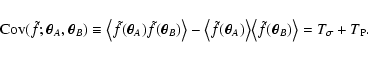
Received 23 January 2002 / Accepted 27 June 2002
Abstract
Interpolation techniques play a central role in Astronomy, where one
often needs to smooth irregularly sampled data into a smooth map.
In a previous article (Lombardi & Schneider 2001, hereafter
Paper I), we have considered a widely used smoothing technique and
we have evaluated the expectation value of the smoothed map under a
number of natural hypotheses. Here we proceed further on this
analysis and consider the variance of the smoothed map, represented
by a two-point correlation function. We show that two main sources
of noise contribute to the total error budget and we show several
interesting properties of these two noise terms. The expressions
obtained are also specialized to the limiting cases of low and high
densities of measurements. A number of examples are used to show in
practice some of the results obtained.
Key words: methods: statistical - methods: analytical - methods: data analysis -
gravitational lensing
1 Introduction
Raw astronomical data are very often discrete, in the sense that
measurements are performed along a finite number of directions on the
sky. In many cases, the discrete data are believed to be single
measurements of a smooth underlying field. In such cases, it is
desirable to reconstruct the original field using interpolation
techniques. A typical example of the general situation just described
is given by weak lensing mass reconstructions in clusters of galaxies.
In this case, thousands of noisy estimates of the tidal field of the
cluster (shear) can be obtained from the observed shapes of background
galaxies whose images are distorted by the gravitational field of the
cluster. All these measurements can then be combined to produce a
smooth map of the cluster shear, which in turn is subsequently
converted into a projected density map of the cluster mass
distribution.
One of the most widely used interpolation techniques in Astronomy is
based on a weighted average. More precisely, a positive weight
function, describing the relative weight of a datum at the position
 on the point
 ,
is introduced.
The weight function is often chosen to be of the form
,
is introduced.
The weight function is often chosen to be of the form
 ,
i.e. depends only on the separation
,
i.e. depends only on the separation
 of the two points considered. Normally, w is also a decreasing
function of
in order to ensure that the largest
contributions to the interpolated value at
comes from
nearby measurements. Then, the data are averaged using a weighted
mean with the weights given by the function w. More precisely,
calling
of the two points considered. Normally, w is also a decreasing
function of
in order to ensure that the largest
contributions to the interpolated value at
comes from
nearby measurements. Then, the data are averaged using a weighted
mean with the weights given by the function w. More precisely,
calling  the nth datum obtained at the position
 ,
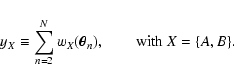
the smooth map is defined as
,
the smooth map is defined as
 |
(1) |
where N is the total number of objects. In a previous paper
(Lombardi & Schneider 2001, hereafter Paper I) we have evaluated
the expectation value for this expression under the following
hypothesis:
In Paper I we have shown that
 |
(5) |
Thus,
 is the convolution of the
unknown field f with an effective weight
is the convolution of the
unknown field f with an effective weight
 which, in general, differs from the weight function w. We also have
shown that
has a "similar'' shape as w and
converges to w when the object density
which, in general, differs from the weight function w. We also have
shown that
has a "similar'' shape as w and
converges to w when the object density  is large; however for
finite ,
is broader than w.
is large; however for
finite ,
is broader than w.
Here we proceed further with the statistical analysis by obtaining an
expression for the two-point correlation function (covariance) of this
estimator. More precisely, given two points
 and
and
 ,
we consider the two-point correlation function of
,
we consider the two-point correlation function of
 ,
defined as
,
defined as
 |
(6) |
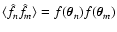
In our calculations, similarly to Paper I, we assume that are unbiased and mutually independent estimates of
 (cf. Eq. (2)). We also assume that the
 have fixed variance
  ,
so that
,
so that
![\begin{displaymath}
\bigl\langle \bigl[ \hat f_n - f(\vec\theta_n) \bigr]
\big...
... f(\vec\theta_m) \bigr] \bigr\rangle = \sigma^2
\delta_{nm} .
\end{displaymath}](/articles/aa/full/2002/36/aa2294/img44.gif) |
(7) |
The paper is organized as follows. In Sect. 2 we
summarize the results obtained in this paper. In
Sect. 3 we derive the general expression for the
covariance of the interpolating techniques and we show that two main
noise terms contribute to the total error. These results are then
generalized in Sect. 4 to include the case
of weight functions that are not strictly positive. A useful
expansion at high densities
of the covariance is obtained in
Sect. 5. Section 6 is
devoted to the study of several interesting properties of the
expressions obtained in the paper. Finally, in
Sect. 7 we consider three simple weight functions and
derive (analytically or numerically) the covariance for these cases.
Four appendixes on more technical topics complete the paper.
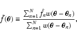
2 Summary
As mentioned in the introduction, the primary aim of this paper is the
evaluation of the covariance (two-point correlation function) of the
smoothing estimator (1) under the hypotheses that
measurements
are unbiased estimates of a field
 (Eq. (2)) and that location measurements
 are independent, uniformly distributed variables with
density .
Hence, we do not allow for angular clustering on the
positions
,
and we also do not include the effects
of a finite field in our calculations (these effects are expected to
play a role on points close to the boundary of the region where data
are available). Moreover, we suppose that the noise on the
measurements
is uncorrelated with the signal (i.e.,
that variance
is constant on the field), and that
measurements are uncorrelated to each other. Finally, we stress that
in the whole paper we assume a non-negative (i.e., positive or
vanishing) weight function
are independent, uniformly distributed variables with
density .
Hence, we do not allow for angular clustering on the
positions
,
and we also do not include the effects
of a finite field in our calculations (these effects are expected to
play a role on points close to the boundary of the region where data
are available). Moreover, we suppose that the noise on the
measurements
is uncorrelated with the signal (i.e.,
that variance
is constant on the field), and that
measurements are uncorrelated to each other. Finally, we stress that
in the whole paper we assume a non-negative (i.e., positive or
vanishing) weight function
 .
Surprisingly,
weight functions with arbitrary sign cannot be studied in our
framework (see discussion at the end of
Sect. 4).
.
Surprisingly,
weight functions with arbitrary sign cannot be studied in our
framework (see discussion at the end of
Sect. 4).
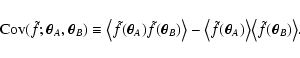
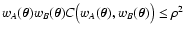
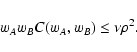
The results obtained in this paper can be summarized in the following
points.
- 1.
- We evaluate analytically the two-point correlation function of
 ,
showing that it is composed of two main
terms:
,
showing that it is composed of two main
terms:
 |
(8) |
The term  is proportional to
and can thus be
interpreted as the contribution to the covariance from measurement
errors; the term
is proportional to
and can thus be
interpreted as the contribution to the covariance from measurement
errors; the term  depends on the signal
and can be interpreted as Poisson noise. These
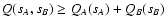
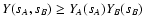
terms can be evaluated using the following set of equations:
depends on the signal
and can be interpreted as Poisson noise. These
terms can be evaluated using the following set of equations:
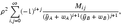
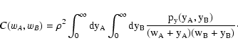
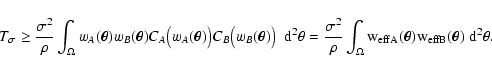
| Q(sA, sB) |
= |
![$\displaystyle \int_\Omega \bigl[ {\rm e}^{-s_A w_A(\vec\theta) -
s_B w_B(\vec\theta)} - 1 \bigr] ~ \rm d^2
\theta ,$](/articles/aa/full/2002/36/aa2294/img49.gif) |
(9) |
| Y(sA, sB) |
= |
![$\displaystyle \exp \bigl[ \rho Q(s_A, s_B) \bigr] .$](/articles/aa/full/2002/36/aa2294/img50.gif) |
(10) |
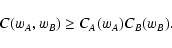
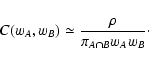
| C(wA, wB) |
= |
 ,$](/articles/aa/full/2002/36/aa2294/img51.gif) |
(11) |
 |
= |
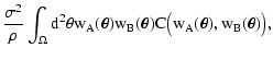 |
(12) |
 |
= |
 |
|
| |
|
![$\displaystyle \times\Bigl[ C\bigl( w_A(\vec\theta_1) +
w_A(\vec\theta_2), w_B(\...
... C_A\bigl( w_A(\vec\theta_1)
\bigr) C_B\bigl( w_B(\vec\theta_2) \bigr) \Bigr] .$](/articles/aa/full/2002/36/aa2294/img56.gif) |
(13) |
In the last two equations we used the notation
 ,
and similarly for
,
and similarly for
 ;
moreover the two functions CA and CB can be obtained from the
following limits:
;
moreover the two functions CA and CB can be obtained from the
following limits:
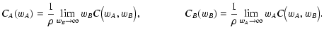 |
|
|
(14) |
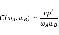
- 2.
- We show that the quantity
C(wA, wB) of Eq. (11), in
the limit of high density ,
converges to
 |
(15) |
where Sij are the moments of the functions
(wA, wB):
![\begin{displaymath}
S_{ij} \equiv \int_\Omega \rm d^2 \theta \bigl[ w_A(\vec\theta)
\bigr]^i \bigl[ w_B(\vec\theta) \bigr]^j .
\end{displaymath}](/articles/aa/full/2002/36/aa2294/img61.gif) |
(16) |
- 3.
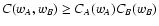
- We derive a number of properties for the noise terms and the
function
C(wA, wB). In particular, we show (1) that
 in every point
;
(2)
that the measurement error has as upper bound
in every point
;
(2)
that the measurement error has as upper bound
 ;
(3) that the same error has as lower bound the
convolution
;
(3) that the same error has as lower bound the
convolution
 of the two
effective weights
of the two
effective weights
 and
and
 (cf. Lombardi & Schneider 2001); (4) that
the measurement noise converges to
(cf. Lombardi & Schneider 2001); (4) that
the measurement noise converges to
 at low
densities (
at low
densities (
 )
and to
)
and to
 at high densities (
 ).
).
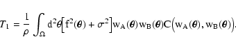
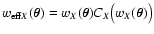
3 Evaluation of the covariance
3.1 Preliminaries
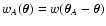
Before starting the analysis, let us introduce a simpler notation. In
the following we will often drop the arguments
and
in
 and
other related quantities. Note, in fact, that the problem is
completely defined with the introduction of the two "shifted'' weight
functions
and
other related quantities. Note, in fact, that the problem is
completely defined with the introduction of the two "shifted'' weight
functions
 and
and
 .
We also call
.
We also call
 and
and
 the values of
at the two points of
interest
and
,
so that
the values of
at the two points of
interest
and
,
so that
 |
(17) |
Hence, Eq. (6) can be rewritten in this notation as
 |
(18) |
Note that, using this notation, we are not taking advantage of the
invariance upon translation of
 in Eq. (1); in
other words, we are not using the fact that wA and wB are
basically the same function shifted by
in Eq. (1); in
other words, we are not using the fact that wA and wB are
basically the same function shifted by
 .
Actually, all calculations can be carried out without using this
property; however, we will explicitly point out simplifications that
can be made using the invariance upon translation.
.
Actually, all calculations can be carried out without using this
property; however, we will explicitly point out simplifications that
can be made using the invariance upon translation.
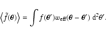
We would also like to spend a few words about averages. Note that, as
anticipated in Sect. 1, we need to carry out two
averages, one with respect to
(Eqs. (2) and
(7)), and one with respect to
(Eqs. (3) and (4)). Taking
to
be random variables is often reasonable because in Astronomy one does
not have a direct control over the positions where observations are
made (this happens because measurements are normally performed in the
direction of astronomical objects such as stars and galaxies, and thus
at "almost random'' directions); it also has the advantage of letting
us obtain general results, independent of any particular configuration
of positions. Note, however, that taking
to be
independent variables is a strong simplification which
might produce inaccurate results in some context (e.g., in case of a
direction dependent density, or in case of clustering; see
Lombardi et al. 2001). Finally, since the number of observations N is
itself a random variable, we need to perform first the average on
and then the one on
 .
.
In closing this section, we observe that in this paper, similarly to
Paper I, we will almost always consider the smoothing problem on the
plane, i.e. we will assume that the positions
are vectors of
 .
We proceed this way because in Astronomy the
smoothing process often takes places on small regions of the celestial
sphere, and thus on sets that can be well approximated with subsets of
the plane. However, we stress that all the results stated here can be
easily applied to smoothing processes that takes places on different
sets, such as the real axis
.
We proceed this way because in Astronomy the
smoothing process often takes places on small regions of the celestial
sphere, and thus on sets that can be well approximated with subsets of
the plane. However, we stress that all the results stated here can be
easily applied to smoothing processes that takes places on different
sets, such as the real axis  or the space
 .
.
3.2 Analytical solution
Let us now focus on the first term on the r.h.s. of
Eq. (18). We have
![\begin{displaymath}
\bigl\langle \tilde f_A \tilde f_B \bigr\rangle = \frac{1}{...
...theta_n) \bigr] \bigl[ \sum_m w_B(\vec\theta_m) \bigr]}
\cdot
\end{displaymath}](/articles/aa/full/2002/36/aa2294/img84.gif) |
(19) |
Note that the average in the r.h.s. of this equation is only with
respect to
.
Expanding the numerator in the integrand
of this equation, we obtain N2 terms, N of which have n = m and
N (N - 1) have  .
We can then rewrite Eq. (19)
above as
.
We can then rewrite Eq. (19)
above as
 |
(20) |
where
![$\displaystyle T_1 \equiv \frac{1}{A^N} \int_\Omega \rm d^2 \theta_1
\int_\Omega...
...bigl[ \sum_n w_A(\vec\theta_n) \bigr] \bigl[
\sum_m w_B(\vec\theta_m) \bigr]} ,$](/articles/aa/full/2002/36/aa2294/img87.gif) |
|
|
(21) |
![$\displaystyle T_2 \equiv \frac{1}{A^N} \int_\Omega \rm d^2 \theta_1
\int_\Omega...
...[ \sum_n
w_A(\vec\theta_n) \bigr] \bigl[ \sum_m w_B(\vec\theta_m) \bigr]}
\cdot$](/articles/aa/full/2002/36/aa2294/img88.gif) |
|
|
(22) |
Despite the apparent differences, these two terms can be simplified in
a similar manner. Let us consider first T1. Using
Eq. (7), we can evaluate the average
![$\langle \hat f^2_n
\rangle = \sigma^2 + \bigl[ f(\vec\theta_n) \bigr]^2$](/articles/aa/full/2002/36/aa2294/img89.gif) .
Since the
positions
appear as "dummy variables'' in
Eq. (21), we can relabel them as follows
.
Since the
positions
appear as "dummy variables'' in
Eq. (21), we can relabel them as follows
![\begin{displaymath}
T_1 = \frac{N}{A^N} \int_\Omega \rm d^2 \theta_1 \int_\Omeg...
...theta_n) \bigr] \bigl[
\sum_m w_B(\vec\theta_m) \bigr]} \cdot
\end{displaymath}](/articles/aa/full/2002/36/aa2294/img90.gif) |
(23) |
In order to simplify this equation, we use a technique similar to the
one adopted in Paper I. More precisely, we split the two sums in the
denominator of the integrand of Eq. (23), taking away the
terms
 and
and
 .
Hence, we write
.
Hence, we write
 |
(24) |
where
C(wA, wB) is a corrective factor given by
![\begin{displaymath}
C(w_A, w_B) \equiv \frac{N^2}{A^{N+1}} \int_\Omega \rm d^2
...
...gr] \bigl[w_B + \sum_{m=2}^N
w_B(\vec\theta_n) \bigr]} \cdot
\end{displaymath}](/articles/aa/full/2002/36/aa2294/img94.gif) |
(25) |
The additional factor
 has been introduced to simplify
some of the following equations. Note that in the definition of CwA and wB are formally taken to be two real variables (instead
of two real functions of argument
has been introduced to simplify
some of the following equations. Note that in the definition of CwA and wB are formally taken to be two real variables (instead
of two real functions of argument
 ).
).
The definition of C above suggests to define two new random
variables yA and yB:
 |
(26) |
Note that the sum runs from n = 2 to n = N. If we could evaluate
the combined probability distribution function
py(yA,
yB) for yA and yB, we would have solved our problem: In fact
we could use this probability to write
C(wA, wB) as follows
 |
(27) |
To obtain the probability distribution
py(yA, yB), we need to use
the combined probability distribution
pw(wA, wB) for wA and
wB. This distribution is implicitly defined by saying that the
probability that
 be in the range
![$[ w_A, w_A + \rm d
w_A ]$](/articles/aa/full/2002/36/aa2294/img99.gif) and
be in the range
and
be in the range
![$[ w_B, w_B + \rm dw_B
]$](/articles/aa/full/2002/36/aa2294/img100.gif) is
is
 .
We can evaluate
pw(wA, wB) using
.
We can evaluate
pw(wA, wB) using
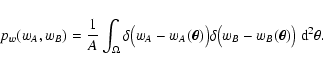 |
(28) |
Turning back to
(yA, yB), we can write a similar expression for
py:
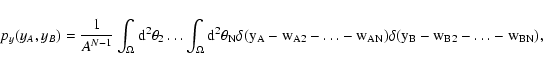 |
(29) |
where for simplicity we have called
 .
Note that inserting this equation into Eq. (27) we recover
Eq. (25), as expected. Actually, for our purposes it is more
useful to consider yX to be the sum of N random variables
.
Note that inserting this equation into Eq. (27) we recover
Eq. (25), as expected. Actually, for our purposes it is more
useful to consider yX to be the sum of N random variables
 .
In other words, we consider the set of couples
.
In other words, we consider the set of couples
 ,
made of the two weight functions at the
various positions, as a set of N independent
two-dimensional random variables
(wA, wB) with probability
distribution
pw(wA, wB). (Hence, similarly to Eq. (25),
we consider the weight functions wX to be real variables instead of
real functions; the independence of the positions
then
implies the independence of the couples
(wAn,
wBn)). Taking this point of view, we can rewrite
Eq. (29) as
,
made of the two weight functions at the
various positions, as a set of N independent
two-dimensional random variables
(wA, wB) with probability
distribution
pw(wA, wB). (Hence, similarly to Eq. (25),
we consider the weight functions wX to be real variables instead of
real functions; the independence of the positions
then
implies the independence of the couples
(wAn,
wBn)). Taking this point of view, we can rewrite
Eq. (29) as
It is well known in Statistics that the sum of independent random
variables with the same probability distribution can be better studied
using Markov's method (see, e.g., Chandrasekhar 1989; see
also Deguchi & Watson 1987 for an application to microlensing
studies). This method is based on the use of Fourier transforms for
the probability distributions pw and py. However, since we are
dealing with non negative quantities (we recall that we assumed
), we can replace the Fourier transform with
Laplace transform which turns out to be more appropriate in for our
problem (see Appendix D for a summary of the
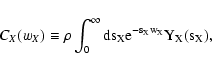
properties of Laplace transforms). Hence, we define
W(sA, sB) and
Y(sA, sB) to be the Laplace transforms of
pw(wA, wB) and
py(wA, wB), respectively. Note that, since both functions pwand py have two arguments, we need two arguments for the Laplace
transforms as well:
 = \int_0^\infty \rm dw_A
\int_0^\infty \rm dw_B {\rm e}^{-s_A w_A - s_B w_B} p_w(w_A, w_B) ,$](/articles/aa/full/2002/36/aa2294/img110.gif) |
|
|
(31) |
 = \int_0^\infty \rm dy_A
\int_0^\infty \rm dy_B {\rm e}^{-s_A y_A - s_B y_B} p_y(y_A, y_B) .$](/articles/aa/full/2002/36/aa2294/img111.gif) |
|
|
(32) |
We use now in these expressions the Eq. (28) for pw and
Eq. (30) for py, thus obtaining
| W(sA, sB) |
= |
 |
(33) |
| Y(sA, sB) |
= |
![$\displaystyle \frac{1}{A^{N-1}} \int_\Omega \! \rm d^2
\theta_2 \dots \int_\Ome...
...^N w_{An} - s_B \sum_{m=2}^N w_{Bm} \biggr] = \bigl[
W(s_A, s_B) \bigr]^{N-1} .$](/articles/aa/full/2002/36/aa2294/img113.gif) |
(34) |
Hence, py can in principle be obtained from the following scheme.
First, we evaluate
W(sA, sB) using Eq. (33), then we
calculate
Y(sA, sB) from Eq. (34), and finally we
back-transform this function to obtain
py(yA, yB).
Actually, another, more convenient, technique is viable. Following
the path of Paper I, we now take the "continuous limit'' and treat
N as a random variable. As explained in
Sect. 1, we can take this limit using two
equivalent approaches:
- We keep the area A fixed and consider N to be a random
variable with Poisson distribution given by Eq. (3). We
then average over all possible configurations obtained.
- We take the limit
 taking the density
fixed.
taking the density
fixed.
The equivalence of the two methods can be shown as follows. Let us
consider a large area
 ,
and let us suppose that the
number
,
and let us suppose that the
number
 of objects inside A' is fixed. Since objects
are randomly distributed inside A', the probability for each object
to fall inside A is just A / A'. Hence N, the number of objects
inside A, follows a binomial distribution:
of objects inside A' is fixed. Since objects
are randomly distributed inside A', the probability for each object
to fall inside A is just A / A'. Hence N, the number of objects
inside A, follows a binomial distribution:
 |
(35) |
If we now let N' go to infinity with
 fixed, the
probability distribution for N converges (see, e.g. Eadie et al. 1971)
to the Poisson distribution in Eq. (3).
fixed, the
probability distribution for N converges (see, e.g. Eadie et al. 1971)
to the Poisson distribution in Eq. (3).
We will follow here the second strategy, i.e. we will take the limit
 keeping
constant. In the limit
keeping
constant. In the limit
 the quantity
W(sA, sB) goes to unity and
thus is not useful for our purposes. Instead, it is convenient to
define
the quantity
W(sA, sB) goes to unity and
thus is not useful for our purposes. Instead, it is convenient to
define
![\begin{displaymath}
Q(s_A, s_B) \equiv \int_\Omega \bigl[ {\rm e}^{-s_A w_A(\ve...
...1 \bigr] ~ \rm d^2 \theta = A \bigl[
W(s_A, s_B) - 1 \bigr] .
\end{displaymath}](/articles/aa/full/2002/36/aa2294/img121.gif) |
(36) |
This definition is sensible because, this way, Q remains finite for
.
In the continuous limit, Eq. (34)
becomes
![\begin{displaymath}
Y(s_A, s_B) = \lim_{N \rightarrow \infty} \left[ 1 + \frac{\rho
Q(s_A, s_B)}{N} \right]^{N-1} = {\rm e}^{Q(s_A, s_B)} .
\end{displaymath}](/articles/aa/full/2002/36/aa2294/img122.gif) |
(37) |
In order to evaluate
C(wA, wB), we rewrite its definition (27) as
 |
(38) |
where
 and
and
 |
(39) |
Here
 are Heaviside functions at the positions
wX, i.e.
are Heaviside functions at the positions
wX, i.e.
 |
(40) |
Note that  is basically a "shifted'' version of py.
Looking back at Eq. (38), we can interpret the integration
present in this equation as a very particular case of
Laplace transform with vanishing argument. In other words, we can
write
is basically a "shifted'' version of py.
Looking back at Eq. (38), we can interpret the integration
present in this equation as a very particular case of
Laplace transform with vanishing argument. In other words, we can
write
 .
\end{displaymath}](/articles/aa/full/2002/36/aa2294/img129.gif) |
(41) |
Thus our problem is solved if we can obtain the Laplace transform of
 evaluated at
sA = sB = 0. From the properties
of Laplace transform (cf. Eq. (D.7)) we find
evaluated at
sA = sB = 0. From the properties
of Laplace transform (cf. Eq. (D.7)) we find
 = \int_{s...
...ty \rm d
s'_A \int_{s_B}^\infty \rm ds'_B ~ Z_w(s'_A, s'_B) ,
\end{displaymath}](/articles/aa/full/2002/36/aa2294/img131.gif) |
(42) |
where Zw is the Laplace transform of :
 = {\rm e}^{-s_A w_A - s_B w_B}
Y(s_A, s_B) .
\end{displaymath}](/articles/aa/full/2002/36/aa2294/img132.gif) |
(43) |
Combining together Eqs. (41)-(43) we finally obtain
 .
\end{displaymath}](/articles/aa/full/2002/36/aa2294/img133.gif) |
(44) |
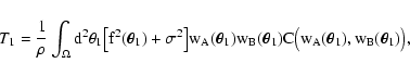
In summary, the set of equations that can be used to evaluate T1are
![\begin{displaymath}
Q(s_A, s_B) = \int_\Omega \bigl[ {\rm e}^{-s_A w_A(\vec\theta)
- s_B w_B(\vec\theta)} - 1 \bigr] ~ \rm d^2 \theta ,
\end{displaymath}](/articles/aa/full/2002/36/aa2294/img134.gif) |
(45) |
![\begin{displaymath}
Y(s_A, s_B) = \exp \bigl[ \rho Q(s_A, s_B) \bigr] ,
\end{displaymath}](/articles/aa/full/2002/36/aa2294/img135.gif) |
(46) |
 ,
\end{displaymath}](/articles/aa/full/2002/36/aa2294/img136.gif) |
(47) |
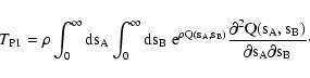
 |
(48) |
These equations solve completely the first part of our problem,
the determination of T1.
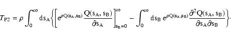
Let us now consider the second term of Eq. (20), namely T2(see Eq. (22)). We first evaluate the average in
that appears in the numerator of the integrand of
Eq. (22), obtaining
 (cf. Eq. (7) with ). Then we relabel the "dummy'' variables
similarly to what has been done for T1, thus obtaining
(cf. Eq. (7) with ). Then we relabel the "dummy'' variables
similarly to what has been done for T1, thus obtaining
![\begin{displaymath}
T_2 = \frac{N (N - 1)}{A^N} \int_\Omega \rm d^2 \theta_1 ~
...
...theta_n) \bigr] \bigl[
\sum_m w_B(\vec\theta_m) \bigr]} \cdot
\end{displaymath}](/articles/aa/full/2002/36/aa2294/img139.gif) |
(49) |
We now split, in the two sums in the denominator, the terms
 and
and
 and define the new random variables
 |
(50) |
Again, if we know the combined probability distribution
pz(zA, zB) of zA and zB our problem is solved, since we can
write (cf. Eqs. (24) and (27))
 |
|
|
(51) |
Actually, in the continuous limit, zX is indistinguishable from
yX (zX differs from yX only on the fact that it is the sum of
N-2 "weights'' instead of N-1; however, N goes to infinity in
the continuous limit and thus yX and zX converge to the same
quantity). Thus we can rewrite Eq. (51) as
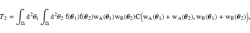 |
(52) |
where C is still given by Eq. (47).
Finally, in order to evaluate
 ,
we still need the
simple averages
,
we still need the
simple averages
 and
and
 .
These can be obtained
directly using the technique described in Paper I, where we have shown
that the set of equations to be used is
.
These can be obtained
directly using the technique described in Paper I, where we have shown
that the set of equations to be used is
![\begin{displaymath}Q_X(s_X) \equiv \int_\Omega \bigl[ {\rm e}^{-s_X
w_X(\vec\theta)} - 1 \bigr] \; ~ \rm d^2 \theta ,
\end{displaymath}](/articles/aa/full/2002/36/aa2294/img148.gif) |
(53) |
![\begin{displaymath}Y_X(s_X) \equiv \exp \bigl[ \rho Q_X(s_X) \bigr] ,
\end{displaymath}](/articles/aa/full/2002/36/aa2294/img149.gif) |
(54) |
 |
(55) |
 |
(56) |
We recall that in Paper I we called the combination
 effective weight (cf.
Eq. (5) in the introduction). Alternatively, we can use the
quantities
Y(sA, sB) and
C(wA, wB) to calculate the correcting
factors CA and CB. From Eqs. (53) and (54) we
immediately find
effective weight (cf.
Eq. (5) in the introduction). Alternatively, we can use the
quantities
Y(sA, sB) and
C(wA, wB) to calculate the correcting
factors CA and CB. From Eqs. (53) and (54) we
immediately find
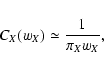
| QA(sA) |
= |
 |
(57) |
| QB(sB) |
= |
 |
(58) |
Then, using the properties of Laplace transforms (cf.
Eq. (D.10)), and comparing the definition of
C(wA, wB)(Eq. (44)) with the one of CX(wX) (Eq. (55)) we
find
|
|
|
(59) |
We now have at our disposal the complete set of equations that can be
used to determine the covariance of .
In closing this subsection we makes a few comments on the translation
invariance for wX (see Sect. 3.1). Since
and
differ by an angular shift
only, the two functions QA and QB are the same, so that CAcoincides with CB. Not surprisingly, the two effective weights
 and
and
 differ also only by a
shift.
differ also only by a
shift.
3.3 Noise contributions
A simple preliminary analysis of the Eqs. (48) and (52)
allows us to recognize two main sources of noise. In
fact, a term in Eq. (48) is proportional to ,
and
is clearly related to measurement errors of f, namely
 |
(60) |
Other factors entering
can be interpreted as Poisson
noise. Hence, we call
 ,
,
 ,
and
,
and
 ,
so that
the total Poisson noise is
,
so that
the total Poisson noise is
 .
Note that the Poisson noise
,
in contrast with the measurement noise ,
strongly depends on the signal
.
.
Note that the Poisson noise
,
in contrast with the measurement noise ,
strongly depends on the signal
.
The noise term
is quite intuitive and does not require a
long explanation. We note here only that this term is independent of
the field
because we assumed measurements with fixed variance
(see Eq. (7)).
The Poisson noise
can be better understood with a
simple example. Suppose that
is not
constant and let us focus on a point where this function has a strong
gradient. Then, when measuring
in this point, we could
obtain an excess of signal because of an overdensity of objects in the
region where
is large; the opposite happens if we have
an overdensity of objects in the region where
is
small. This noise source, called Poisson noise, vanishes if the
function
is flat.
In the rest of this paper we will study the properties of the
two-point correlation function. Before proceeding, however, we need
to consider an important generalization of the results obtained here
to the case of vanishing weights.
4 Vanishing weights
So far we have implicitly assumed that both wA and wB are always
positive. In some cases, however, it might be interesting to consider
vanishing weight functions (for example, functions with finite
support). We need then to modify accordingly our equations.
When using vanishing weights, we might encounter situations where the
denominator of Eq. (1) vanishes because all weight functions
 vanish as well. In this case, the
estimator
cannot be even defined (we encounter
the ratio 0 / 0), and any further statistical analysis is
meaningless. In practice, when smoothing data using a vanishing
weight function, one could just ignore the points
where
the smoothed function
is not defined, i.e. the
points
for which
vanish as well. In this case, the
estimator
cannot be even defined (we encounter
the ratio 0 / 0), and any further statistical analysis is
meaningless. In practice, when smoothing data using a vanishing
weight function, one could just ignore the points
where
the smoothed function
is not defined, i.e. the
points
for which
 for
every n. This simple approach leads to smoothed maps with
"holes'', i.e. defined only on subsets of the plane. Hence, if we
choose this approach we need to modify accordingly the statistical
analysis that we carry out in this paper.
for
every n. This simple approach leads to smoothed maps with
"holes'', i.e. defined only on subsets of the plane. Hence, if we
choose this approach we need to modify accordingly the statistical
analysis that we carry out in this paper.
This problem was already encountered in Paper I, where we used the
following prescription. When using a finite-field weight function, we
discard, for every configuration of measurement points
,
the points
on the plane for which the
smoothing
is not defined. Then, when taking
the average with respect to all possible configurations
of
,
we just exclude these
configurations. We stress that, this way, the averages
 and
and
 of the smoothing (1) at two
different points
and
of the smoothing (1) at two
different points
and
 are effectively
carried out using different ensembles: In one case we exclude the
"bad configurations'' for
,
in the other case the "bad
configurations'' for
.
are effectively
carried out using different ensembles: In one case we exclude the
"bad configurations'' for
,
in the other case the "bad
configurations'' for
.
The same prescription is also adopted here to evaluate the covariance
of our estimator. Hence, when performing the ensemble average to
estimate the covariance
,
we explicitly exclude configurations where either
 or
or
 cannot be evaluated. This is implemented with a slight
change in the definition of py, which in turn implies a change in
Eq. (46) for Y. A rigorous generalization of the relevant
equations can now be carried out without significant difficulties.
However, the equations obtained are quite cumbersome and present some
technical peculiarities. Hence, we prefer to postpone a complete
discussion of vanishing weights until
Appendix A; we report here only the main
results.
cannot be evaluated. This is implemented with a slight
change in the definition of py, which in turn implies a change in
Eq. (46) for Y. A rigorous generalization of the relevant
equations can now be carried out without significant difficulties.
However, the equations obtained are quite cumbersome and present some
technical peculiarities. Hence, we prefer to postpone a complete
discussion of vanishing weights until
Appendix A; we report here only the main
results.
As mentioned above, the basic problem of having vanishing weights is
that in some cases the estimator is not defined. Hence, it is
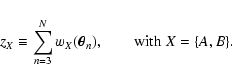
convenient to define three probabilities, namely PA and PB, the
probabilities, respectively, that
and
are
not defined, and PAB, the probability that both quantities are
not defined. Note that, because of the invariance upon translation
for w, we have PA = PB. These probabilities can be estimated
without difficulties. In fact, the quantity
 is not
defined if and only if there is no object inside the support of wX.
Since the number of points inside the support of wX follows a
Poisson probability, we have
is not
defined if and only if there is no object inside the support of wX.
Since the number of points inside the support of wX follows a
Poisson probability, we have
 ,
where
,
where  is the area of the support of wX. Similarly, calling
 the area of the union of the supports of wA and wB, we
find
the area of the union of the supports of wA and wB, we
find
 .
Using Eqs. (45)
and (46) we can also verify the following relations
.
Using Eqs. (45)
and (46) we can also verify the following relations
PAB=![$\displaystyle \lim_{\begin{array}{c}
\scriptstyle s_A \rightarrow \infty \\ [-...
...rrow 0^+ \\ [-1mm]
\scriptstyle s_B \rightarrow 0^+
\end{array}} Y(s_A, s_B) ,$](/articles/aa/full/2002/36/aa2294/img174.gif) |
(61) |
PA=![$\displaystyle \lim_{\begin{array}{c}
\scriptstyle s_A \rightarrow 0^+ \\ [-2mm...
...w \infty \\ [-1mm]
\scriptstyle s_B \rightarrow 0^+
\end{array}} Y(s_A, s_B) .$](/articles/aa/full/2002/36/aa2294/img175.gif) |
(62) |
Appendix A better clarifies the
relationship between the limiting values of Y and the probabilities
defined above. In the following we will use a simplified notation for
limits, and we will write something like
 for
the left equation in (62).
for
the left equation in (62).
The only significant modification to the equations obtained above for
vanishing weights is an overall factor in Eq. (47), which now
becomes
 .
\end{displaymath}](/articles/aa/full/2002/36/aa2294/img177.gif) |
(63) |
The factor
1/(1 - PA - PB + PAB) is basically a
renormalization; more precisely, it is introduced to take into account
the fact that we are discarding cases where either
or
are not defined. Note, in fact, that in agreement with
the inclusion-exclusion principle,
(1 - PA - PB + PAB) is the
probability that the both
and
are defined.
Since the combination
(1 - PA - PB + PAB) enters several
equations, we define
 |
(64) |
Equation (63) is the most important correction to take into
account for vanishing weights. Actually, there are also a number of
peculiarities to consider when dealing with the probability py and
its Laplace transform Y. Fortunately, however, these peculiarities
have no significant consequence for our purpose and thus we can still
safely use Eqs. (45) and (46). Again, we refer to
Appendix A for a complete explanation.
In closing this section, we spend a few words on weight functions with
arbitrary sign (i.e., functions
that can be positive,
vanishing, or positive depending on
). As mentioned in
Sect. 2, in this case a statistical study of the
smoothing (1) cannot be carried out using our framework. In
order to understand why this happens, let us consider the weight
function
 |
(65) |
This function is continuous, positive for
 ,
and quickly vanishes for large
,
and quickly vanishes for large
 .
Let us
then consider separately the numerator and denominator of
Eq. (1). The denominator can clearly be positive or
negative; more precisely, the denominator is positive for points
close to at least one of the locations
,
and negative for points
which are in "voids'' (i.e., far
away from the locations
). Hence, the lines where
the denominator vanishes separate the regions of high density of
locations from the regions of low density. Note that, even for very
large average densities ,
we still expect to find "voids'' of
arbitrary size (in other words, for every finite density ,
there
is a non-vanishing probability of having no point inside an
arbitrarily large region). As a result, there will be always regions
where the denominator vanishes. The discussion for the numerator is
similar but, in this case, we also need to take into account the field
.
Hence, we still expect to have regions where the
numerator is positive and regions where it is negative but, clearly,
these regions will in general be different from the analogous regions
for the denominator. As a result, when evaluating the ratio between
the numerator and the denominator, we will obtain arbitrarily large
values close to the lines where the denominator vanishes. Note also
that these lines will change for different configurations of locations
.
In summary, if the weight function is allowed
to be negative, the denominator of Eq. (1) is no longer
guaranteed to be positive, and infinities are expected when performing
the ensemble average.
.
Let us
then consider separately the numerator and denominator of
Eq. (1). The denominator can clearly be positive or
negative; more precisely, the denominator is positive for points
close to at least one of the locations
,
and negative for points
which are in "voids'' (i.e., far
away from the locations
). Hence, the lines where
the denominator vanishes separate the regions of high density of
locations from the regions of low density. Note that, even for very
large average densities ,
we still expect to find "voids'' of
arbitrary size (in other words, for every finite density ,
there
is a non-vanishing probability of having no point inside an
arbitrarily large region). As a result, there will be always regions
where the denominator vanishes. The discussion for the numerator is
similar but, in this case, we also need to take into account the field
.
Hence, we still expect to have regions where the
numerator is positive and regions where it is negative but, clearly,
these regions will in general be different from the analogous regions
for the denominator. As a result, when evaluating the ratio between
the numerator and the denominator, we will obtain arbitrarily large
values close to the lines where the denominator vanishes. Note also
that these lines will change for different configurations of locations
.
In summary, if the weight function is allowed
to be negative, the denominator of Eq. (1) is no longer
guaranteed to be positive, and infinities are expected when performing
the ensemble average.
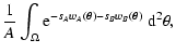
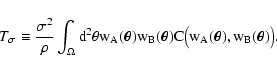
5 Moments expansion
In most applications, the density of objects is rather large. Hence,
it is interesting to obtain an expansion for
C(wA, wB) valid at
high densities.
In Paper I we already obtained an expansion for CA(wA) (or,
equivalently, CB(wB)) for
:
 |
(66) |
In this equation, Sij are the moments of the functions
(wA,
wB), defined as
| |
(67) |
Clearly, in Eq. (66) enter only the moments Si0, since the
form of wB is not relevant for CA(wA). Similarly, the
expression for CB(wB) contains only the moments S0j. Note
that for weight functions invariant upon translation we have
Sij =
Sji.
![\begin{figure}
\includegraphics[width=14cm,clip]{2294f1.eps}\end{figure}](/articles/aa/full/2002/36/aa2294/Timg183.gif) |
Figure 1:
The moment expansion of
C(wA, wB) for
1-dimensional Gaussian weight functions
wA(x) = wB(x) centered on 0 and with unit variance. The plot shows the
various order approximations obtained using the method
described in Sect. 5 (equations for
the orders n=3 and n=4 are not explicitly reported in the
text; see however Table B.1 in
Appendix B). The density used is
 . . |
| Open with DEXTER |
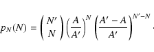
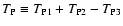
![\begin{figure}
\parbox[t]{1.5\hsize}{%
\hskip-1.5mm\resizebox{\hsize}{!}{%
\input fig5.tex}
}
\end{figure}](/articles/aa/full/2002/36/aa2294/Timg185.gif) |
Figure 2:
The function
C(wA, wB) is
monotonically decreasing with wA and wB, while
wA wB
C(wA, wB) (scaled in this plot) is monotonically
increasing. The parameters used for this figure are the same
as Fig. 1. Note that, since
PA = PB = 0, we
have
 in
agreement with Eqs. (82) and (83); moreover
in
agreement with Eqs. (82) and (83); moreover
 as expected from
Eq. (84).
as expected from
Eq. (84). |
| Open with DEXTER |
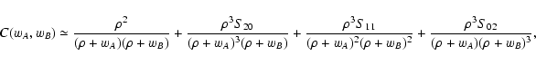
A similar expansion can be obtained for
C(wA, wB). Calculations
are basically a generalization of what was done in Paper I for C(w)and can be found in Appendix B. Here we
report only the final result obtained:
 |
|
|
(68) |
We note that using this expansion and Eqs. (59) we can
recover the first terms of Eq. (66), as expected.
Figure 1 shows the results of applying this expansion
to a Gaussian weight. For clarity, we have considered in this figure
(and in others shown below) a 1-dimensional smoothing instead of the
2-dimensional case discussed in the text, and we have used x as
spatial variable instead of
.
The figure refers to two
identical Gaussian weight functions with vanishing average and unit
variance. A comparison of this figure with Fig. 2 of Paper I shows
that the convergence here is much slower. Nevertheless,
Eq. (68) will be very useful to investigate some important
limiting cases in the next section.
6 Properties
In this section we will study in detail the two noise terms and
introduced in Sect. 3.3,
showing their properties and considering several limiting cases. The
results obtained are of clear interest of themselves; for example, we
will derive here upper and lower limits for the measurement error
that can be used at low and high densities. Moreover, this
section helps us understand the results obtained so far, and in
particular the peculiarities of vanishing weights.
6.1 Normalization
A simple normalization property for
C(wA, wB) can be derived,
similarly to what we have already done for the average of in Paper I. Suppose that
 and that no errors are
present on the measurements, so that
and that no errors are
present on the measurements, so that
 .
In this case we
will always measure
.
In this case we
will always measure
 (see Eq. (1)),
so that
(see Eq. (1)),
so that
 ,
,
 ,
and no error is expected on .
This
result can be also recovered using the analytical expressions obtained
so far. Let us first consider the simpler case of non-vanishing
weights.
,
and no error is expected on .
This
result can be also recovered using the analytical expressions obtained
so far. Let us first consider the simpler case of non-vanishing
weights.
Using Eqs. (47) and (48), we can write the term
 in the case
as
in the case
as
 |
(69) |
The last integrand in this equation can be rewritten as
 (cf. the definition of Q,
Eq. (45)):
(cf. the definition of Q,
Eq. (45)):
 |
(70) |
Analogously, for
 we obtain (cf. Eq. (52))
We can integrate this expression by parts taking
![$\rho {\rm e}^{\rho Q} ~
(\partial Q / \partial s_B) = \bigl[ \partial \exp(\rho Q) / \partial
s_B \bigr]$](/articles/aa/full/2002/36/aa2294/img200.gif) as differential term:
as differential term:
 |
(72) |
We now observe that the last term in Eq. (72) is identical to
what we founded in Eq. (70). Hence, the sum
 is
is
The last equation holds because, for non-vanishing weights,
Y(0+,
0+) = 1 and all other terms vanishes (cf.
Eqs. (61)-(62)). Hence, as expected,
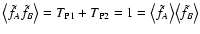 .
.
In case of vanishing weights, we can still use Eqs. (70)
and (72) with an additional factor  (due to the
extra factor in Eq. (63)). The last step in
Eq. (73) thus now becomes
(due to the
extra factor in Eq. (63)). The last step in
Eq. (73) thus now becomes
![\begin{displaymath}
T_{\rm P1} + T_{\rm P2} = \nu \bigl[ Y(\infty, \infty) -
Y(\infty, 0^+) - Y(0^+, \infty) + Y(0^+, 0^+) \bigr] = 1 .
\end{displaymath}](/articles/aa/full/2002/36/aa2294/img208.gif) |
(74) |
The last equality holds since now Y does not vanishes for large
(sA, sB) (see again Eqs. (61)-(62)).
6.2 Scaling
Similarly to what was already shown in Paper I, for all expressions
encountered so far some scaling invariance properties hold.
First, we note that, although we have assumed that the weight
functions wA and wB are normalized to unity, all results are
clearly independent of their actual normalization. Hence, a trivial
scaling property holds: All results (and in particular the final
expression for
)
are left unchanged by the
transformation
 or,
equivalently,
or,
equivalently,
 |
|
|
(75) |
A more interesting scaling property is the following. Consider the
transformation
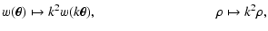 |
|
|
(76) |
where both factors k2 must be changed according to the dimension of
the
vector space. If we apply this transformation, then
the expression for
is transformed according to
 |
(77) |
This invariance suggests that the shape of
is
controlled by the expected number of objects for which the two weight
functions are significantly different from zero. Hence, similarly to
what done in Paper I, we define the two weight areas
 and
and
 as
as
![\begin{displaymath}
\mathcal{A}_X \equiv \biggl[ \int_\Omega \bigl[
w_X(\vec\t...
...[2mm]
S_{02}^{-1}\quad {\rm if} \ X = B .
\end{array}\right.
\end{displaymath}](/articles/aa/full/2002/36/aa2294/img215.gif) |
(78) |
For weight functions invariant upon translation we have
 .
We call
.
We call
 the weight number of objects (again,
 because of the invariance upon translation). Note that
this quantity is left unchanged by the scaling (76). Similar
definitions hold for the effective weight
because of the invariance upon translation). Note that
this quantity is left unchanged by the scaling (76). Similar
definitions hold for the effective weight
 and the effective number of objects
 .
.
6.3 Behavior of C
In order to better understand the properties of C, it is useful to
briefly consider its behavior as a function of the weights wA and wB.
We observe that, since
Y(sA, sB) > 0 for every
(sA, sB) (see
Eq. (46)),
C(wA, wB) decreases if either wA or wBincrease. In order to study the behavior of the quantity
wA wB
C(wA, wB) that enters the noise term T1, we consider the
quantity
wA C(wA, wB):
![\begin{displaymath}
w_A C(w_A, w_B) = \nu \rho^2 \int_{0^-}^\infty \rm ds_B ~
...
..._A} \biggr) {\rm e}^{- s_A w_A}
\biggr] {\rm e}^{- s_B w_B} .
\end{displaymath}](/articles/aa/full/2002/36/aa2294/img221.gif) |
(79) |
This equation can be shown by integrating by parts the integral over
sA. The partial derivative required in Eq. (79) can be
evaluated from Eq. (46):
 |
(80) |
Since this derivative is negative, we can deduce that the integral
over sA in Eq. (79) increases with wA, and thus
wA
C(wA, wB) also increases as wA increases. Similarly, it can be
shown that
wB C(wA, wB) increases as wB increases. In
summary, the quantity
wA wB C(wA, wB) behaves as wA wB, in
the sense that its partial derivatives have the same sign as the
partial derivatives of wA wB (see Fig. 2). Also,
since
C(wA, wB) decreases if either wA or wB increase, we
can deduce that
wA wB C(wA, wB) is "broader'' than wA wB.
Since
 is positive,
the function
is positive,
the function
 shares the same support as
 .
It is also interesting to study the limits of
wA
wB C(wA, wB) at high and low values for wA and wB. From the
properties of Laplace transform (see Eq. (D.10)), we have
.
It is also interesting to study the limits of
wA
wB C(wA, wB) at high and low values for wA and wB. From the
properties of Laplace transform (see Eq. (D.10)), we have
 |
(81) |
where Eq. (61) has been used in the second equality. Hence,
the quantity
wA wB C(wA, wB) goes to zero only if
PAB = 0.
In other cases, we expect a discontinuity at
wA = wB = 0.
Similarly, using Eqs. (61)-(62) we find
Since
wA wB C(wA, wB) increases with both wA and wB, the
last equation above puts a superior limit for this quantity:
 |
(85) |
Suppose that the two points
and
are far
away from each other, so that
is
very close to zero everywhere. In this situation we can greatly
simplify our equations.
If
is far away from
,
then
and
are never significantly
different from zero at the same position
.
In this case,
the integral in the definition of
Q(sA, sB) (see
Eq. (45)) can be split into two integrals that corresponds to
QA and QB (Eq. (53)):
 |
|
|
(86) |
Hence, if the two weight functions wA and wB do not have
significant overlap, the function
C(wA, wB) reduces to the product
of the two correcting functions CA and CB.
In general, it can be shown that
 .
In fact, we have
.
In fact, we have
![\begin{displaymath}
C(w_A, w_B) - C_A(w_A) C_B(w_B) = \rho^2 \int_0^\infty \rm ...
...(s_A, s_B)} - {\rm e}^{\rho Q_A(s_A) + \rho Q_B(s_B)} \bigr] .
\end{displaymath}](/articles/aa/full/2002/36/aa2294/img236.gif) |
(87) |
We now observe that
![\begin{displaymath}
Q(s_A, s_B) - Q_A(s_A) - Q_B(s_B) = \int_\Omega \bigl[ {\rm...
...igr] \bigl[ {\rm e}^{-s_B w_B(\vec\theta)} - 1
\bigr] \ge 0 .
\end{displaymath}](/articles/aa/full/2002/36/aa2294/img237.gif) |
(88) |
Hence,
 and the difference
between the two terms of this inequality is an indication of overlap
between the two weight functions wA and wB. Since the
exponential function is monotonic, we find
and the difference
between the two terms of this inequality is an indication of overlap
between the two weight functions wA and wB. Since the
exponential function is monotonic, we find
 and thus
 |
(89) |
6.5 Upper and lower limits for

The normalization property shown in Sect. 6.1 can
also be used to obtain an upper limit for .
We observe, in
fact, that
is indistinguishable from
 for a constant function
.
This
case, however, has already been considered above in
Sect. 6.1: There we have shown that
for a constant function
.
This
case, however, has already been considered above in
Sect. 6.1: There we have shown that
 .
Since
.
Since
 ,
we find the
relation
.
,
we find the
relation
.
The property just obtained has a simple interpretation. As shown by
Eq. (60),
is proportional to  and thus we
would expect that this quantity is unbounded superiorly. In reality,
even when we are dealing with a very small density of objects, the
estimator (1) "forces'' us to use at least one object. This
point has already been discussed in Paper I, where we showed that the
number of effective objects,
and thus we
would expect that this quantity is unbounded superiorly. In reality,
even when we are dealing with a very small density of objects, the
estimator (1) "forces'' us to use at least one object. This
point has already been discussed in Paper I, where we showed that the
number of effective objects,
 ,
is always
larger than unity. The upper limit found for
can be
interpreted using the same argument. Note that this result also holds
for weight functions with finite support.
,
is always
larger than unity. The upper limit found for
can be
interpreted using the same argument. Note that this result also holds
for weight functions with finite support.
A lower limit for ,
instead, can be obtained from the
inequality (89):
 |
(90) |
Hence, the error
is larger than a convolution of the two
effective weight functions. In case of finite-field weight functions,
the limit just obtained must be corrected with a factor .
The
argument to derive Eq. (90) is then slightly more complicated
because of the presence of the PX probabilities. However, using
the relation
 ,
we can recover Eq. (90)
with the aforementioned corrective factor.
,
we can recover Eq. (90)
with the aforementioned corrective factor.
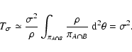
6.6 Limit of low and high densities
In the limit
we can obtain simple expressions for
the noise terms. If
vanishes, we have
Y(sA, sB) = 1 (cf.
Eq. (46)) and thus
 |
(91) |
In this equation we have assumed
wA wB > 0. Note that we have
reached here the superior limit indicated by Eq. (85). In
the same limit,
,
 and
and
 ,
where
,
where
 is the area of the intersection of the
supports of wA and wB. Hence we find
is the area of the intersection of the
supports of wA and wB. Hence we find
 |
(92) |
Analogously, in the same limit, we have found in Paper I
 |
(93) |
where wX > 0 has been assumed. We can then proceed to evaluate the
various terms. For
we obtain the expression
 |
(94) |
Note that the integral has been evaluated only on the subset of the
plane where
wA wB > 0; the case where this product vanishes, in
fact, need not to be considered because the quantity
wA wB C(wA,
wB) vanishes as well. Exactly the same result holds for weight
functions with infinite support. Hence, when
we
reach the superior limit discussed in
Sect. 6.5 for .
Equation (94) can be better appreciated with the following
argument. As the density
approaches zero, the probability of
having two objects on
vanishes. Because of the
prescription regarding vanishing weights (cf. beginning of
Sect. 4), the ensemble average in our limit
is performed with one and only one object in
 .
Since
we have only one object, this is basically used with unit weight in
the average (17), and thus the measurement noise is just given
by
.
Since
we have only one object, this is basically used with unit weight in
the average (17), and thus the measurement noise is just given
by
 .
.
Let us now consider the limit at low densities of the Poisson noise,
which, we recall, has been split into three terms,
,
,
and
 (see
Sect. 3.3). Inserting Eq. (92)
into Eq. (24), we find for
(see
Sect. 3.3). Inserting Eq. (92)
into Eq. (24), we find for
 |
(95) |
where
 denotes the
simple average of f2 on the set
.
Hence,
converges to the average of f2 on the intersection
of the supports of wA and wB. Again, we can explain this result
using an argument similar to the one used for Eq. (94).
Regarding
,
we observe that this term is of
first order in
because
C(wA, wB) is of first order (cf.
Eqs. (92) and (52)). We can then safely ignore this
term in our limit
.
Finally, as shown in Paper I,
at low densities the expectation value for
is a simple
average of f on the support of wX, i.e.
denotes the
simple average of f2 on the set
.
Hence,
converges to the average of f2 on the intersection
of the supports of wA and wB. Again, we can explain this result
using an argument similar to the one used for Eq. (94).
Regarding
,
we observe that this term is of
first order in
because
C(wA, wB) is of first order (cf.
Eqs. (92) and (52)). We can then safely ignore this
term in our limit
.
Finally, as shown in Paper I,
at low densities the expectation value for
is a simple
average of f on the support of wX, i.e.
 .
Hence,
.
Hence,
 and the Poisson
noise in the limit of small densities is given by
and the Poisson
noise in the limit of small densities is given by
 |
(96) |
In case of a constant function
,
this expression
vanishes as expected. Surprisingly, in general, we cannot say that
 .
Rather, if
.
Rather, if
 ,
and if in particular
the two weight functions have different supports, we might have a
negative .
Suppose, for example, that f vanishes on
the intersection of the two supports
,
but is
otherwise positive. In this case, the first term in the r.h.s. of
Eq. (96) vanishes, while the second term contributes with a
negative sign, and thus
,
and if in particular
the two weight functions have different supports, we might have a
negative .
Suppose, for example, that f vanishes on
the intersection of the two supports
,
but is
otherwise positive. In this case, the first term in the r.h.s. of
Eq. (96) vanishes, while the second term contributes with a
negative sign, and thus
 .
On the other hand, if
wA = wB then
has to be non-negative.
.
On the other hand, if
wA = wB then
has to be non-negative.
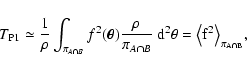
We now consider the opposite limiting case, namely high density. In
this case, it is useful to use the moment expansion (68).
Since
and
have an overall factor in its definition (cf. Eq. (60)), we can simply take the
0th order for
C(wA, wB), thus obtaining
 |
|
|
(97) |
For
and
,
instead, we need to use a
first order expansion in
for
C(wA, wB). This can be done
by using the first terms in series (66), and by expanding all
fractions in terms of powers of .
Inserting the result into
the definitions of
and
we obtain
Note that we have dropped, in these equations, terms of order higher
than .
The difference
 is
is
![\begin{displaymath}
T_{\rm P2} - T_{\rm P3} \simeq \frac{1}{\rho}
\int_\Omega ...
...\bigl[ S_{11} - w_A(\vec\theta_2) - w_B(\vec\theta_1) \bigr] .
\end{displaymath}](/articles/aa/full/2002/36/aa2294/img273.gif) |
(100) |
Using Eqs. (100) and (97), we can verify that
vanishes if f is constant, as expected:
where the normalization of w has been used. Also, it is apparent
that all noise sources, including Poisson noise, are proportional to
at high densities.
In order to further investigate the properties of Poisson noise at
high densities, we write it in a more compact form. Let us define the
average of a function
 weighted with
 as
as
![\begin{displaymath}
\langle g \rangle_q \equiv \biggl[ \int_\Omega g(\vec\theta...
... \biggl[ \int_\Omega
q(\vec\theta) ~ \rm d^2 \theta \biggr] .
\end{displaymath}](/articles/aa/full/2002/36/aa2294/img279.gif) |
(102) |
Using this definition we can rearrange Eqs. (97) and
(100) in the form
![\begin{displaymath}
T_{\rm P} = \frac{S_{11}}{\rho} \Bigl[ \bigl\langle f^2
\b...
...f \rangle_{w_A
w_B} - \langle f \rangle_{w_B} \bigr) \Bigr] .
\end{displaymath}](/articles/aa/full/2002/36/aa2294/img280.gif) |
(103) |
This expression suggests that the Poisson noise is actually made of
two different terms,
 and
and
 .
The
first term is proportional to the difference between two averages of
f2 and f; both averages are performed using wA wB as weight.
Hence, this term is controlled by the "internal scatter'' of f on
points where both weight functions are significantly different from
zero; it is always positive. The second term is made of averages fusing different weight functions. It can be either positive or
negative if
.
Actually, as already seen in the limiting
case
,
the overall Poisson noise does not need to
be positive, and anti-correlation can be present in some cases.
.
The
first term is proportional to the difference between two averages of
f2 and f; both averages are performed using wA wB as weight.
Hence, this term is controlled by the "internal scatter'' of f on
points where both weight functions are significantly different from
zero; it is always positive. The second term is made of averages fusing different weight functions. It can be either positive or
negative if
.
Actually, as already seen in the limiting
case
,
the overall Poisson noise does not need to
be positive, and anti-correlation can be present in some cases.
6.7 Limit of high and low frequencies
The strong dependence of the Poisson noise on the function
makes an analytical estimate of this noise
contribution extremely difficult in the general case. However, it is
still possible to study the behavior of
in two important
limiting cases, that we now describe.
Suppose that the function
does not change
significantly on the scale length of the weight functions
and
(or, in other words, that the
power spectrum of f has a peak at significantly lower frequencies
than the power spectra of wA and wB). In this case, we can take
the function f as a constant in the integrals of Eq. (13),
and apply the results of Sect. 6.1. Hence, in the
limit of low frequencies, the Poisson noise vanishes.
Suppose now, instead, that the function
does not have
any general trend on the scale length of the weight
functions, but that instead changes at significantly smaller scales
(again, this behavior is better described in terms of power spectra:
We require here that the power spectrum of f has a peak at high
frequencies, while it vanishes for the frequencies where the power
spectra of wA and wB are significantly different from zero).
In this case, we can assume that integrals such as
 |
|
|
(104) |
vanish approximately, because the average of f on large scales
vanishes (remember that we are assuming that f has no general trend
on large scales). Similarly, the integrals that appear in
and
vanish as well. In this case, then, the only
contribution to the Poisson noise arises from
.
This can be
easily evaluated
 |
(105) |
where we have denoted with
 the
average of |f|2 on large scales. Hence we finally obtain
the
average of |f|2 on large scales. Hence we finally obtain
 |
(106) |
The results discussed in this section can also be numerically verified
in simple cases. Figure 8, for example, shows the Poisson
noise expected in the measurement of a periodic field when using
two Gaussian weight functions (see Sect. 7.2 for details).
From this figure, we see that the Poisson noise increases with the
frequency of the field f, and quickly attains a maximum value at
high frequencies. Moreover, the same figure shows that, in agreement
with Eq. (106), the Poisson noise at the maximum is simply
related to the measurement noise
(cf. Fig. 7 for
 ).
).
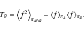
7 Examples
Similarly to what has been done in Paper I, in this section we
consider three typical weight functions, namely a top-hat, a Gaussian,
and a parabolic weight. For simplicity, we will consider
1-dimensional cases only; this will have also some advantages when
representing the results obtained with figures. Hence, we will use
x instead of
as spatial variable.
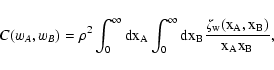
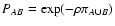
7.1 Top-hat
![\begin{figure}
\includegraphics[width=14cm,clip]{2294f3.eps} \end{figure}](/articles/aa/full/2002/36/aa2294/Timg287.gif) |
Figure 3:
The value of
 for top-hat weights as a
function of the density .
Both weight functions wA and
wB are top-hats (see Eq. (107)) centered on zero.
Using Eq. (108), we can use this graph to obtain
as a function of the density and the point separation
xA - xB.
for top-hat weights as a
function of the density .
Both weight functions wA and
wB are top-hats (see Eq. (107)) centered on zero.
Using Eq. (108), we can use this graph to obtain
as a function of the density and the point separation
xA - xB. |
| Open with DEXTER |
![\begin{figure}
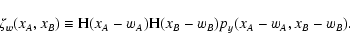
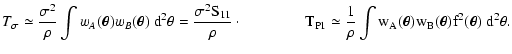
\includegraphics[width=14cm,clip]{2294f4.eps} \end{figure}](/articles/aa/full/2002/36/aa2294/Timg288.gif) |
Figure 4:
The noise term
for two top-hat weights as a
function of the point separation
 for
two densities,
and
for
two densities,
and  .
The plot also shows
the quantity .
The plot also shows
the quantity
 ,
which at high densities
approximates
(since then ,
which at high densities
approximates
(since then
 ). Note that
S11 for a top-hat function is just given by ). Note that
S11 for a top-hat function is just given by
 . . |
| Open with DEXTER |
The simplest weight that we can consider is a top-hat function,
defined as
![\begin{displaymath}
w(x) =
\left\{\begin{array}{l}
1 \quad {\rm if} \ \vert x...
...< 1/2 , \\ [2mm]
0 \quad {\rm otherwise.}
\end{array}\right.
\end{displaymath}](/articles/aa/full/2002/36/aa2294/img289.gif) |
(107) |
Since w is either 1 or 0, we just need to consider C(1,1) to
evaluate .
Regarding the Poisson noise, from
Eq. (52) we deduce that C(1,2), C(2,1), and C(2,2) are
also required.
Figure 3 shows C(1,1) and
as functions of
the density
for two identical top-hat weight functions centered
on the origin. From this plot we can recognize some of the limiting
cases studied above. In particular, the fact that
goes
to unity at low densities is related to Eq. (92); similarly,
the limit of C(1,1) at high densities is consistent with
Eq. (68). The same figure shows also the moments expansion
of C(1,1) up to forth order. As expected, the expansion completely
fails at low densities, while is quite accurate for  .
.
Curves in Fig. 3 have been calculated using the standard
approach described by Eqs. (45), (46) and
(63). Actually, in the simple case of top-hat weight
functions, we can evaluate C(1,1) using a more direct statistical
argument. We start by observing that in our case, for xA = xB, we have
 |
(108) |
On the other hand, a top-hat weight function is basically acting by
taking simple averages for all objects that fall inside its support.
This suggests that, for xA = xB, we can evaluate its measurement
noise as
 |
(109) |
where p(N) is the probability of having N objects inside the
support. This probability is basically a Poisson probability
distribution with average .
However, since we are adopting the
prescription of "avoiding'' weight functions without objects in their
support, we must explicitly discard the case N = 0 and consequently
renormalize the probability. In summary, we have
![\begin{displaymath}
p(N) = \frac{{\rm e}^{-\rho} \rho^N}{N!} \biggm/ \bigl[ 1 - {\rm e}^{-\rho}
\bigr] .
\end{displaymath}](/articles/aa/full/2002/36/aa2294/img293.gif) |
(110) |
This expression combined with Eq. (109) allows us to evaluate
 :
:
 |
(111) |
We can directly verify this result using Eqs. (45),
(46) and (63). In fact, for the top-hat function we
find
| Q(sA, sB) |
= |
![$\displaystyle \bigl[ {\rm e}^{-s_A -s_B} - 1 \bigr] ,$](/articles/aa/full/2002/36/aa2294/img296.gif) |
(112) |
| Y(sA, sB) |
= |
 |
(113) |
| C(1, 1) |
= |
 |
|
| |
= |
 |
(114) |
Finally, with a change of the dummy variable
 we
recover Eq. (111).
we
recover Eq. (111).
![\begin{figure}
\includegraphics[width=14cm,clip]{2294f5.eps} \end{figure}](/articles/aa/full/2002/36/aa2294/Timg301.gif) |
Figure 5:
Numerical calculations for 1-dimensional
Gaussian weight functions wA = wB centered on 0 and with
unit variance. The various curves shows the function
wA wB
C(wA, wB) for different densities .
Note that, as
expected,
C(wA, wB) approaches unity for largedensities. |
| Open with DEXTER |
![\begin{figure}
\includegraphics[width=14cm,clip]{2294f6.eps} \end{figure}](/articles/aa/full/2002/36/aa2294/Timg302.gif) |
Figure 6:
Same as Fig. 5, but for two Gaussian weight
functions centered on 0 and 1 and with unit variance. |
| Open with DEXTER |
![\begin{figure}\includegraphics[width=14cm,clip]{2294f7.eps} \end{figure}](/articles/aa/full/2002/36/aa2294/Timg303.gif) |
Figure 7:
The noise term
for two Gaussian weights (of
unit variance) as function of their separation. Similarly to
Fig. 4, the plot also shows the high-density
approximations
.
Note that in this case S11 is also a Gaussian (with double variance). |
| Open with DEXTER |
![\begin{figure}
\includegraphics[width=14cm,clip]{2294f8.eps} \end{figure}](/articles/aa/full/2002/36/aa2294/Timg306.gif) |
Figure 8:
The Poisson noise TP for two Gaussian weights (of unit
variance) for a periodic function of the form
 as a function of the weight separation
,
for a density .
Note that, as expected, the Poisson
noise increases with k and approaches the limit discussed in
Sect. 6.7 for high frequencies. More
precisely, since for a sine function we have
as a function of the weight separation
,
for a density .
Note that, as expected, the Poisson
noise increases with k and approaches the limit discussed in
Sect. 6.7 for high frequencies. More
precisely, since for a sine function we have
 ,
Eq. (106) gives ,
Eq. (106) gives
 (this can indeed be verified by a comparison with
Fig. 7). Note also that, while TP is strictly
positive for
(this can indeed be verified by a comparison with
Fig. 7). Note also that, while TP is strictly
positive for
 ,
it can became negative (see curve for
k = 0.5) at larger separations. ,
it can became negative (see curve for
k = 0.5) at larger separations. |
| Open with DEXTER |
The other terms needed for the Poisson noise can be evaluated using a
calculation similar to the one performed in Eq. (114).
Actually, it can be shown that for any positive integers wA and
wB we have
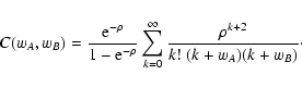 |
(115) |
Figure 4 shows the expected measurement noise
as
a function of the point separation
.
Note that,
for densities of order
or larger, a good approximation is
obtained by just taking
C(wA, wB) = 1 (cf. the moments expansion
(68)), so that
 ;
we also
observe that, for a top-hat weight function, S11 is a linear
function.
;
we also
observe that, for a top-hat weight function, S11 is a linear
function.
7.2 Gaussian
Frequently, a Gaussian weight function of the form
 |
(116) |
is used. Although it is not possible to carry out analytical
calculations and obtain
C(wA, wB), numerical integrations do not
pose any problem. Figure 5 shows, for different densities,
the function
wA wB C(wA, wB) for two identical weights wA =
wB centered in zero; Fig. 6 shows the same quantity when
one of the weight function is centered at unity. Note that, in this
last figure, the largest covariance is at x = 0.5, as expected.
Figure 7 shows the expected measurement noise
as
a function of the weight separation. Similarly to the top-hat weight,
an approximation valid for high density is
 .
Figure 8 shows, instead, the Poisson noise
expected
for a field f of the form
,
for different values of
k. Note that the noise, as expected, increases with k, and
quickly reaches the "saturation'' value discussed in
Sect. 6.7. Note also that the noise is, at lowest
lowest density, negative for
.
Figure 8 shows, instead, the Poisson noise
expected
for a field f of the form
,
for different values of
k. Note that the noise, as expected, increases with k, and
quickly reaches the "saturation'' value discussed in
Sect. 6.7. Note also that the noise is, at lowest
lowest density, negative for
 .
.
7.3 Parabolic weight
![\begin{figure}
\includegraphics[width=14cm,clip]{2294f9.eps} \end{figure}](/articles/aa/full/2002/36/aa2294/Timg312.gif) |
Figure 9:
Numerical calculations for 1-dimensional
parabolic weight functions wA = wB centered on 0 and with
unit variance. The various curves shows the function
wA wB
C(wA, wB) for different densities . |
| Open with DEXTER |
![\begin{figure}
\includegraphics[width=14cm,clip]{2294f10.eps} \end{figure}](/articles/aa/full/2002/36/aa2294/Timg313.gif) |
Figure 10:
The noise term
for two parabolic weights as a
function of their separation (see also Figs. 4 and
7). |
| Open with DEXTER |
Finally, we study of a parabolic weight function of the form
![\begin{displaymath}
w(x) =
\left\{\begin{array}{l}
3 x^2 / 4 \quad {\rm if} \...
..., \\ [2mm]
0 \qquad\quad {\rm otherwise.}
\end{array}\right.
\end{displaymath}](/articles/aa/full/2002/36/aa2294/img314.gif) |
(117) |
This function illustrates well some of the peculiarities of finite
support weight functions. Figure 9 shows the results of
numerical integrations for
wA wB C(wA, wB) at different
densities .
A first interesting point to note is the
discontinuity observed at x = 1, which is in agreement with
Eq. (81). Moreover, as expected from Eq. (92), the
function plotted clearly approaches a constant at low densities
.
Finally, the measurement noise
is plotted in
Fig. 10.
8 Conclusions
In this article we have studied in detail the covariance of a widely
used smoothing technique. The main results obtained are summarized in
the following items.
- 1.
- The covariance is composed of two main terms,
and
,
representing measurement errors and Poisson noise,
respectively; the latter one depends on the field f on which the
smoothing is performed.
- 2.
- Expressions to compute
and
have been
provided. In particular, it has been shown that both terms can be
obtained in term of a kernel
C(wA, wB), which in turn can be
evaluated from the weight function
.
- 3.
- We have obtained an expansion of the kernel
C(wA, wB) valid
at high densities .
- 4.
- We have shown that
has an upper limit, given by
,
and a lower limit, provided by Eq. (90).
- 5.
- We have evaluated the form of the noise contributions in the
limiting cases of high and low densities.
- 6.
- We have considered three typical cases of weight functions and
we have evaluated
C(wA, wB) for them.
Finally, we note that although the smoothing technique considered in
this paper is by far the most widely used in Astronomy, alternative
methods are available. A statistical characterization of these
methods, using a completely different approach, will be presented in a
future paper (Lombardi & Schneider, in preparation).
Acknowledgements
This work was partially supported by a grant from
the Deutsche Forschungsgemeinschaft, and the TMR Network
"Gravitational Lensing: New constraints on Cosmology and the
Distribution of Dark Matter.''
Appendix A: Vanishing weights
In Sect. 3.2 we have obtained the solution
of the covariance problem under the hypothesis that the weight
function
is strictly positive. In this appendix we
will generalize the results obtained there to non-negative weight
functions (see also Sect. 4).
If wA is allowed to vanish, then we might have a finite probability
that yA vanishes, i.e. a finite probability that no point
is inside the support of wA. A finite probability
in a probability distribution function appears as a Dirac's delta
distribution. Since this point is quite important for our discussion,
let us make a simple example. Suppose that  is a real random
variable with the following characteristics:
is a real random
variable with the following characteristics:
-
has probability 1/3 to vanish.
-
has probability 2/3 to be in the range
 ;
in
this range
has an exponential distribution.
;
in
this range
has an exponential distribution.
Then we can write the probability distribution function for as
 |
(A.1) |
where  is the Heaviside function (see Eq. (40)).
In other words, the probability distribution for
includes the
contribution from a Dirac's delta distribution centered on
is the Heaviside function (see Eq. (40)).
In other words, the probability distribution for
includes the
contribution from a Dirac's delta distribution centered on  .
If
.
If  is known, the probability that
is exactly zero (1/3in this example) can be obtained using
is known, the probability that
is exactly zero (1/3in this example) can be obtained using
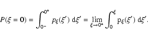 |
(A.2) |
Let us now turn to our problem. As mentioned above, for vanishing
weights we expect that yA might vanish, i.e. its probability might
include the contribution from a delta distribution centered on yA =
0; similarly, if wB is allowed to vanish, the probability
distribution for yB might include a delta centered in yB = 0.
For a given yB, the probability PA(yB) that yA vanishes is
given by
 ,
\end{displaymath}](/articles/aa/full/2002/36/aa2294/img322.gif) |
(A.3) |
where the properties of Laplace transform have been used in the last
equality (see Appendix D). A similar
equation holds for the probability that yB vanishes, PB(yA).
Note that the Laplace transform in Eq. (A.3) is performed only
with respect to the first variable. The joint probability PABthat both yA and yB vanish is (cf. Eq. (61))
 =
Y(\infty, \infty) .
\end{displaymath}](/articles/aa/full/2002/36/aa2294/img323.gif) |
(A.4) |
We then also define (cf. Eqs. (62))
Using Eq. (45), we find
 ,
,
 ,
and
,
where
,
and
,
where
 is the area of the support of wA,
  is the area of
the support of wB, and
is the area of the union of
the two supports. This result is of course not surprising and has
been already derived in the paragraph before Eq. (61) using a
different approach.
is the area of
the support of wB, and
is the area of the union of
the two supports. This result is of course not surprising and has
been already derived in the paragraph before Eq. (61) using a
different approach.
For vanishing weights, we decided to use the following prescription:
We discard, in the ensemble average for
,
the configurations
for which the
function
is not defined either at
or at
.
In order to implement this prescription, we can
explicitly modify the probability distribution py and exclude "by
hand'' cases where the denominator of Eq. (19) vanishes; for
the purpose, we consider separately cases where wA or wB vanish.
We define a new probability distribution for
(yA, yB) which
accounts for vanishing weights:
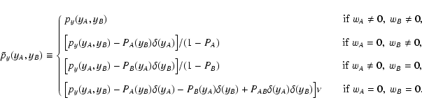 |
(A.7) |
We recall that
 .
In constructing
this probability, first we have explicitly removed the degenerate
situations, then we have renormalized the resulting probability. Note
that the normalization factor in the last case, namely
1 - PA - PB
+ PAB, comes from the so-called "inclusion-exclusion principle''
(
1 - PA - PB + PAB is the probability that both
fA and fB are defined). Using this new probability
distribution in the definition (32) for Y we obtain
.
In constructing
this probability, first we have explicitly removed the degenerate
situations, then we have renormalized the resulting probability. Note
that the normalization factor in the last case, namely
1 - PA - PB
+ PAB, comes from the so-called "inclusion-exclusion principle''
(
1 - PA - PB + PAB is the probability that both
fA and fB are defined). Using this new probability
distribution in the definition (32) for Y we obtain
 |
(A.8) |
Finally, we need to change the normalization factor in
Eq. (47) in order to account for cases where yA or yBare vanishing. Indeed, the correcting factor
C(wA, wB) has been
obtained by assuming that all objects can populate all the plane with
uniform probability distribution (cf. Eq. (25)); now,
however, a fraction
(PA + PB - PAB) of configurations have been
excluded. Hence we have
| |
(A.9) |
This complete the discussion of vanishing weights.
Appendix B: Moments expansion
In Sect. 5 we have written the moments
expansion for
C(wA, wB). Here we complete the discussion by
providing a proof for that result.
At high densities, yA and yB are basically Gaussian random
variables with average values  and
and  (we anticipate
here that these averages are given by the density ). Hence, we
can expand them in the definition of
C(wA, wB):
(we anticipate
here that these averages are given by the density ). Hence, we
can expand them in the definition of
C(wA, wB):
where Mij are the "centered'' moments of py:
 |
(B.2) |
The centered moments can be expressed in terms of the "un-centered''
ones, defined as
 |
(B.3) |
Here
Y(i,j)(0, 0) is the ith partial derivative on sA and
jth partial derivative on sB of
Y(sA, sB), evaluated at (0,
0). These, in turn, can be expressed as derivatives of Q. For the
first terms we have
| Y(0,0)(0,0) |
= |
 |
(B.4) |
| Y(2,0)(0,0) |
= |
![$\displaystyle \rho Q^{(2,0)}(0,0) + \bigl[ \rho Q^{(1,0)}
(0,0) \bigr]^2 ,$](/articles/aa/full/2002/36/aa2294/img354.gif) |
(B.5) |
| Y(1,1)(0,0) |
= |
![$\displaystyle \rho Q^{(1,1)}(0,0) + \bigl[ \rho Q^{(1,0)}(0,0)
\bigr] \bigl[ \rho Q^{(0,1)}(0,0) \bigr] ,$](/articles/aa/full/2002/36/aa2294/img355.gif) |
(B.6) |
| Y(0,2)(0,0) |
= |
![$\displaystyle \rho Q^{(0,2)}(0,0) + \bigl[ \rho
Q^{(0,1)}(0,0) \bigr]^2 .$](/articles/aa/full/2002/36/aa2294/img356.gif) |
(B.7) |
Finally, the derivatives of Q can be evaluated as
|
Q(i,j)(0, 0) = (-1)i+j Sij ,
|
(B.8) |
where Sij, we recall, is given by Eq. (67). Note that
S01 = S10 = 1 because of the normalization of wA and wB,
and thus, as already anticipated,
 .
In
summary, we find
.
In
summary, we find
| M00 |
= |
 |
(B.9) |
| M11 |
= |
 |
(B.10) |
We stress that, in general, it is not true that
 (more complex expressions are encountered for higher order terms; cf.
the last term in Eq. (66)). Finally, we can write the
expansion of
C(wA, wB):
(more complex expressions are encountered for higher order terms; cf.
the last term in Eq. (66)). Finally, we can write the
expansion of
C(wA, wB):
 |
(B.11) |
This is precisely Eq. (68). Using the same technique and a
little more perseverance, we can also obtain higher order terms. In
particular, Table B.1 reports the moments Mij defined in
Eq. (B.2) up to the forth order. This table, together with
Eq. (B.1), can be used to write an accurate moment expansion
of
C(wa, wB).
Appendix C: Varying weights
In Paper I we have considered a modified version of the estimator
(1) which allows for the use of supplementary weights.
Suppose that we measure a given field
at some
positions
of the sky. Suppose also that we use a
weight un for each object observed, so that we replace
Eq. (1) with
 |
(C.1) |
For example, if we have at our disposal some error estimate  for each object, we might use the weighting scheme
 in order to minimize the noise of the estimator
(C.1).
in order to minimize the noise of the estimator
(C.1).
A statistical study of the expectation value of this estimator has
already been carried out in Paper I. Here we proceed further and
study its covariance under the same assumptions as the ones used for
the study of Eq. (1) in the main text. However, since one of
the main reasons to use weights is some knowledge on the variance of
each object, we use a generalized form of Eq. (7):
![\begin{displaymath}
\bigl\langle \bigl[ \hat f_n - f(\vec\theta_n) \bigr]
\big...
...ec\theta_m) \bigr] \bigr\rangle = \sigma^2(u_n)
\delta_{nm} .
\end{displaymath}](/articles/aa/full/2002/36/aa2294/img365.gif) |
(C.2) |
Note, in particular, that the variance is assumed to depend on un(or, equivalently, the weight is assumed to depend on the variance).
Similarly to Paper I, we also assume that, for each object n, the
weight un is independent of the position
and of the
measured signal ,
and that each un follows a known
probability distribution pu.
In Paper I we have shown that the average value of
can be calculated using the equations
| RX(sX) |
 |
![$\displaystyle \int_\Omega \rm d^2 \theta \int_0^\infty \rm du
~ p_u(u) \bigl[ {...
...-s_X u w_X(\vec\theta)} - 1 \bigr] = \int_0^\infty
p_u(u) Q_X(u s_X) ~ \rm du ,$](/articles/aa/full/2002/36/aa2294/img366.gif) |
(C.3) |
| YX(sX) |
|
![$\displaystyle \exp\bigl[ \rho R_X(s_X) \bigr] ,$](/articles/aa/full/2002/36/aa2294/img367.gif) |
(C.4) |
| BX(vX) |
|
 ,$](/articles/aa/full/2002/36/aa2294/img368.gif) |
(C.5) |
 |
= |
 |
(C.6) |
We now evaluate the covariance of the estimator (C.1) using a
technique similar to the one used in Sect. 3. We have
![\begin{displaymath}
\bigl\langle \tilde f_A \tilde f_B \bigr\rangle = \frac{1}{...
...a_n) \bigr] \bigl[ \sum_m u_m w_B(\vec\theta_m) \bigr]}
\cdot
\end{displaymath}](/articles/aa/full/2002/36/aa2294/img371.gif) |
(C.7) |
As usual we consider separately the cases n = m and ,
thus
obtaining the two terms T1 and T2:
| T1 |
= |
![$\displaystyle \frac{N}{A^N} \int_\Omega \rm d^2 \theta_1 \int_0^\infty
\rm du_1...
...um_n u_n w_A(\vec\theta_n) \bigr] \bigl[
\sum_m u_m w_B(\vec\theta_m) \bigr]} ,$](/articles/aa/full/2002/36/aa2294/img372.gif) |
(C.8) |
| T2 |
= |
![$\displaystyle \frac{N (N - 1)}{A^N} \int_\Omega \rm d^2 \theta_1
\int_0^\infty ...
... u_n w_A(\vec\theta_n) \bigr] \bigl[ \sum_m u_m
w_B(\vec\theta_m) \bigr]} \cdot$](/articles/aa/full/2002/36/aa2294/img373.gif) |
(C.9) |
Let us introduce new variables
 (with
(with
 )
for the combination of weights, and let us define
similarly to Eq. (26)
)
for the combination of weights, and let us define
similarly to Eq. (26)
 .
Then
the probability distributions for vXn and yX can be evaluated
using the set of equations
.
Then
the probability distributions for vXn and yX can be evaluated
using the set of equations
| pv(vA, vB) |
= |
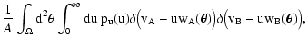 |
(C.10) |
| py(yA, yB) |
= |
 |
|
| |
|
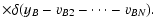 |
(C.11) |
Again, it is convenient to consider the Laplace transforms of these
two probability distributions:
| V(sA, sB) |
= |
 = \frac{1}{A} \int_0^\infty
\rm du ~ p_...
...theta) - s_B u w_B(\vec\theta)} = \int_0^\infty p(u) W(u
s_A, u s_B) ~ \rm du ,$](/articles/aa/full/2002/36/aa2294/img380.gif) |
(C.12) |
| Y(sA, sB) |
= |
 = \bigl[ V(s_A, s_B)
\bigr]^{N-1} .$](/articles/aa/full/2002/36/aa2294/img381.gif) |
(C.13) |
In the continuous limit we define instead
| R(sA, sB) |
|
![$\displaystyle \int_\Omega \rm d^2 \theta \int_0^\infty
\rm du ~ p_u(u) \bigl[ {...
...u
w_B(\vec\theta)} - 1 \bigr] = \int_0^\infty p_u(u) Q(u s_A, u s_B) ~
\rm du ,$](/articles/aa/full/2002/36/aa2294/img382.gif) |
(C.14) |
| Y(sA, sB) |
= |
![$\displaystyle \exp\bigl[ \rho R(s_A, s_B) \bigr] .$](/articles/aa/full/2002/36/aa2294/img383.gif) |
(C.15) |
Finally, the equivalent of the correcting factor
C(wA, wB) (cf. Eq. (11)) is, in our case, the quantity
 .
\end{displaymath}](/articles/aa/full/2002/36/aa2294/img384.gif) |
(C.16) |
The quantity B can be used to evaluate T1: In fact, we
have
| T1 |
= |
![$\displaystyle \frac{N}{A} \int_\Omega \rm d^2 \theta_1 \int_0^\infty
\rm du_1 ~...
...[ u_1
w_A(\vec\theta_1) + y_A \bigr] \bigl[ u_1 w_B(\vec\theta_1) + y_B
\bigr]}$](/articles/aa/full/2002/36/aa2294/img385.gif) |
|
| |
= |
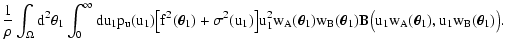 |
(C.17) |
Similarly, for T2 we obtain
| T2 |
= |
 |
|
| |
|
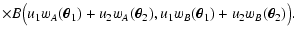 |
(C.18) |
The final evaluation of
then proceeds similarly to
what done in the main text for the estimator (1).
Appendix D: Properties of the Laplace transform
For the convenience of the reader, we summarize in this appendix some
useful properties of the Laplace transform. Proofs of the results
stated here can be found in any advanced analysis book
(e.g. Arfken 1985). Although in this paper we have been dealing
mainly with Laplace transforms of two-argument functions, we write the
properties below for the case of a function of a single argument for
two main reasons: (i) The generalization to functions of several
arguments is in most cases trivial; (ii) Several properties can be
better understood in the simpler case considered here.
Suppose that a function f(x) of a real argument x is given. Its
Laplace transform is defined as
 \equiv {} \lim_{x \rightarrow 0^-} \int_x^...
...e}^{-s x'} = \int_{0^-}^\infty \rm dx ~ f(x) {\rm e}^{-s x}
.
\end{displaymath}](/articles/aa/full/2002/36/aa2294/img389.gif) |
(D.1) |
Note that we use 0- as lower integration limit in this definition.
The Laplace transform is a linear operator; hence, if
 and
and  are two real numbers and g(x) is a function of
real argument x, we have
are two real numbers and g(x) is a function of
real argument x, we have
![$\mathcal L[\alpha f + \beta g] = \alpha \mathcal L[f] +
\beta \mathcal L[g]$](/articles/aa/full/2002/36/aa2294/img392.gif) .
.
The Laplace transform of the derivative of f can be expressed in
terms of the Laplace transform of f. In particular, we have
 = s \mathcal L[f](s) - f(0^-) .
\end{displaymath}](/articles/aa/full/2002/36/aa2294/img393.gif) |
(D.2) |
This equation can be generalized to higher order derivatives. Calling
f(n) the nth derivative of f, we have
 = s^n \mathcal L[f](s) - \sum_{i=0}^{n-1}
s^{n-i-1} f^{(n)}(0^-) .
\end{displaymath}](/articles/aa/full/2002/36/aa2294/img394.gif) |
(D.3) |
Surprisingly, this equation holds if, for n negative, we consider
f(n) to be the -nth integral of f; note that in this case
the summation disappears. Hence, for example, we have
 = \frac{1}{s}
\mathcal L[f](s) .
\end{displaymath}](/articles/aa/full/2002/36/aa2294/img395.gif) |
(D.4) |
Often, properties of the Laplace transform come in pairs: For every
property there is a similar one where the role of f and
![$\mathcal L[f]$](/articles/aa/full/2002/36/aa2294/img396.gif) are
swapped. Here is the "dual'' of property (D.2):
are
swapped. Here is the "dual'' of property (D.2):
 = - \frac{\rm d\mathcal L[f](s)}{\rm ds} ,
\end{displaymath}](/articles/aa/full/2002/36/aa2294/img397.gif) |
(D.5) |
or, more generally,
 = (-1)^n \frac{\rm d^n \mathcal L[f](s)}{\rm d
s^n} \cdot
\end{displaymath}](/articles/aa/full/2002/36/aa2294/img398.gif) |
(D.6) |
A similar equation holds for "negative'' derivatives, i.e. integrals
of the Laplace transform. In this case, however, it is convenient to
change the integration limits to
 .
In summary, we can
write
.
In summary, we can
write
 = \int_s^\infty \mathcal L[f](s') ~ \rm ds'
.
\end{displaymath}](/articles/aa/full/2002/36/aa2294/img400.gif) |
(D.7) |
Given a positive number a, the Laplace transform of the function fshifted by a is given by
 = \mathcal L[f](s) {\rm e}^{- s a}
,
\end{displaymath}](/articles/aa/full/2002/36/aa2294/img401.gif) |
(D.8) |
where
is the Heaviside function defined in
Eq. (40). A dual of this property can also be written:
 = \mathcal L[f](s - b) .
\end{displaymath}](/articles/aa/full/2002/36/aa2294/img402.gif) |
(D.9) |
Finally, we consider two useful relationships between limiting values
of f and
:
 .$](/articles/aa/full/2002/36/aa2294/img403.gif) |
|
|
(D.10) |
-
Arfken, G. 1985, Mathematical methods for physicists (Orlando, Florida:
Academic press)
In the text
-
Chandrasekhar, S. 1989, Stochastic, statistical, and hydromagnetic problems
in physics and astronomy (Chicago: University of Chicago Press, c1989)
In the text
-
Deguchi, S., & Watson, W. D. 1987, Phys. Rev. Lett., 59, 2814
In the text
NASA ADS
-
Eadie, W., Drijard, D., James, F., Roos, M., & Sadoulet, B. 1971, Statistical
Methods in Experimental Physics (Amsterdam New-York Oxford: North-Holland
Publishing Company)
In the text
-
Lombardi, M., & Schneider, P. 2001, A&A, 373, 359
NASA ADS
-
Lombardi, M., Schneider, P., & Morales-Merlino, C. 2001, A&A, 382, 769
In the text
NASA ADS
Copyright ESO 2002
![\begin{figure}
\includegraphics[width=14cm,clip]{2294f1.eps}\end{figure}](/articles/aa/full/2002/36/aa2294/img183.gif)
![\begin{figure}
\parbox[t]{1.5\hsize}{%
\hskip-1.5mm\resizebox{\hsize}{!}{%
\input fig5.tex}
}
\end{figure}](/articles/aa/full/2002/36/aa2294/img185.gif)
![\begin{figure}
\includegraphics[width=14cm,clip]{2294f3.eps} \end{figure}](/articles/aa/full/2002/36/aa2294/img287.gif)
![\begin{figure}
\includegraphics[width=14cm,clip]{2294f4.eps} \end{figure}](/articles/aa/full/2002/36/aa2294/img288.gif)
![\begin{figure}
\includegraphics[width=14cm,clip]{2294f5.eps} \end{figure}](/articles/aa/full/2002/36/aa2294/img301.gif)
![\begin{figure}
\includegraphics[width=14cm,clip]{2294f6.eps} \end{figure}](/articles/aa/full/2002/36/aa2294/img302.gif)
![\begin{figure}\includegraphics[width=14cm,clip]{2294f7.eps} \end{figure}](/articles/aa/full/2002/36/aa2294/img303.gif)
![\begin{figure}
\includegraphics[width=14cm,clip]{2294f8.eps} \end{figure}](/articles/aa/full/2002/36/aa2294/img306.gif)
![\begin{figure}
\includegraphics[width=14cm,clip]{2294f9.eps} \end{figure}](/articles/aa/full/2002/36/aa2294/img312.gif)
![\begin{figure}
\includegraphics[width=14cm,clip]{2294f10.eps} \end{figure}](/articles/aa/full/2002/36/aa2294/img313.gif)

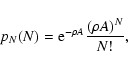


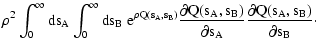
![$\displaystyle \biggr[ \rho \int_0^\infty
\rm ds_A ~ {\rm e}^{\rho Q(s_A, s_B)} ...
...ho {\rm e}^{\rho Q(s_A, s_B)} \biggr]_{s_A = 0}^\infty \biggr]_{s_B =
0}^\infty$](/articles/aa/full/2002/36/aa2294/img204.gif)
![$\displaystyle \lim_{\begin{array}{c}
\scriptstyle w_A \rightarrow \infty \\ [-1mm]
\scriptstyle w_B \rightarrow 0^+
\end{array}} w_A w_B
C(w_A, w_B)$](/articles/aa/full/2002/36/aa2294/img227.gif)
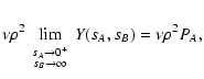
![$\displaystyle \lim_{\begin{array}{c}
\scriptstyle w_A \rightarrow 0^+ \\ [-2mm]
\scriptstyle w_B \rightarrow \infty
\end{array}} w_A w_B
C(w_A, w_B)$](/articles/aa/full/2002/36/aa2294/img229.gif)
![$\displaystyle \nu \rho^2 \lim_{\begin{array}{c}
\scriptstyle s_A \rightarrow \i...
...m]
\scriptstyle s_B \rightarrow 0^+
\end{array}} Y(s_A, s_B) = \nu \rho^2 P_B ,$](/articles/aa/full/2002/36/aa2294/img230.gif)
![$\displaystyle \lim_{\begin{array}{c}
\scriptstyle w_A \rightarrow \infty \\ [-2mm]
\scriptstyle w_B \rightarrow \infty
\end{array}} w_A w_B
C(w_A, w_B)$](/articles/aa/full/2002/36/aa2294/img231.gif)
![$\displaystyle \nu \rho^2 \lim_{\begin{array}{c}
\scriptstyle s_A \rightarrow 0^...
...[-1mm]
\scriptstyle s_B \rightarrow 0^+
\end{array}} Y(s_A, s_B) = \nu \rho^2 .$](/articles/aa/full/2002/36/aa2294/img232.gif)
![$\displaystyle \int_\Omega \rm d^2 \theta_1 \int_\Omega \rm d^2
\theta_2 ~ f(\ve...
...frac{w_B(\vec\theta_2)}{\rho} + \frac{S_{20} + S_{11} +
S_{02}}{\rho} \biggr] ,$](/articles/aa/full/2002/36/aa2294/img269.gif)
![$\displaystyle \int_\Omega \rm d^2 \theta_1 \int_\Omega
\rm d^2 \theta_2 ~ f(\ve...
...} -
\frac{w_B(\vec\theta_2)}{\rho} + \frac{S_{20} + S_{02}}{\rho}
\biggr] \cdot$](/articles/aa/full/2002/36/aa2294/img271.gif)
 = Y(\infty, 0^+) ,$](/articles/aa/full/2002/36/aa2294/img325.gif)
 = Y(0^+, \infty) .$](/articles/aa/full/2002/36/aa2294/img326.gif)

![$\displaystyle \rho^2 \int_0^\infty \rm dy_A \int_0^\infty \rm dy_B
\frac{p_y(y_...
...sum_{j=0}^\infty \left( \frac{\bar
y_B - y_B}{w_B + \bar y_B} \right)^j \biggr]$](/articles/aa/full/2002/36/aa2294/img349.gif)