3 Comparisons

   
3.1 Occultations

Two successful occultations of Kleopatra have been reported by a few observers (Dunham 1981,1992). In Fig. 1 the predicted shape of Kleopatra based on the radar model is plotted against the chords of the 1980 and 1991 occultations. The plots in Fig. 1 are given in the plane of the occultation, i.e. the plane perpendicular to the direction of the occulted star as seen from the asteroid. If no error were present in the predicted position of the star and the asteroid, the images would be centered in the graph origin. Thus the error of the predicted occultation path is of the order of 100 km in 1991. Error bars on the occultation chords, as derived from a timing error of $\pm0.5$ s for visual observations, are of the order of 15 km; for photoelectric observations they reduce to $\sim$3 km. One isolated point, not constraining a chord length and in clear disagreement with nearby chords has been omitted in the 1980 occultation plot. Also one chord of the 1991 event, probably affected by a strong dating error of the emersion point, has been removed from the plot. Negative observations (i.e. observations for which no occultation was detected) are indicated by dashed lines. They put some limits in Kleopatra's size and shape during the 1991 event. The superposition of the model's profile to the observed occultation chords in Fig. 1, is obtained by a translation of the physical model, along the abscissa and ordinate axes (X and Y), such that the predicted contour fits most of the immersion and emersion points. The sub-Earth point longitude was $160\hbox{$^\circ$ }$ and $120\hbox{$^\circ$ }$, during the 1980 and 1991 occultation, respectively. Longitudes of $90\hbox{$^\circ$ }$ and $180\hbox{$^\circ$ }$ correspond roughly to lightcurve maximum and minimum, respectively.

The topographic model was originally scaled in size to the occultations chords. From Fig. 1 we infer that Kleopatra's shape model is in general good agreement with the observed chords. The largest discrepancies are of the order of 30 km, well within the error bars of the model. Despite the inherent difficulty of obtaining robust occultation data, it must be noted that the overall size of the contour on its most elongated direction is well constrained in the 1991 event by a photoelectric chord or by two independent and consistent chords. Hence, based mainly on the 1991 data, it cannot be excluded that a more elongated topographic model could provide a better fit to the measured chords, without drastic change to the 1980 plot.

Figure 1: Comparison between the observed occultation data and the radar model. Left panel: occultation of Oct. 10, 1980 at 7.00 h UTC. Right panel: occultation of Jan. 1, 1991 at 5.28 h UTC. The dashed lines correspond to negative observations. Error bars are given by crosses and are negligible for the photoelectric observations.

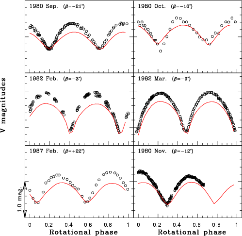
Figure 2: Observed and computed lightcurves for (216) Kleopatra at nearly equatorial views ($\beta$ is the SEP latitude). The curves for the computed values correspond to the radar model with a Minnaert law (k=0.6, see text).

   
3.2 Lightcurves

Many lightcurves of Kleopatra at different geometries were obtained during the last decades. Since the rotation period is known with good accuracy, no shift in the position of the extrema is observed. Figure 2 shows the comparison of the nominal radar model to the photometric observations acquired at large aspect angle (i.e. close to an equatorial view), assuming a homogeneous albedo distribution (Hammergren et al. 2000). Calculation of the global flux depends on the resolution of the topographic model. The radar model is provided with a resolution in spherical coordinates better than $5\times5~\deg^2$, which provides enough internal accuracy for comparison to typical lightcurves. Synthetic lightcurves are constructed by considering the size and orientation - with respect to the Earth and the Sun - of the illuminated and visible elementary surface (the facets for a topographic model). For non-convex shapes like Kleopatra, one also needs to take into account shadows cast by facets and hidden facets. Moreover the computed lightcurves in Fig. 2 were obtained by considering the moderate limb-darkening effect (Minnaert law with k=0.6) mentioned in Sect. 2.

It appears in Fig. 2 that the computed lightcurves do not reproduce the large amplitude of the observed ones. This could be due to the choice of the limb-darkening parameter, since the higher the limb-darkening, the larger the amplitude of the curve. However, we have verified that even using the largest possible Lambertian center-to-limb darkening - which is typical of icy satellites and shall not be realistic for a M-type asteroid - the amplitude would still be underestimated in some cases by about 20%. This suggests that, assuming a moderate limb-darkening parameter, either important albedo variations are present on both ends of Kleopatra's surface, or its actual shape is likely to be more elongated with dimensions ratio of the order of $a/b \sim 2.8$, hence consistent with the error-bars of the model ( $a/b \sim 2.3\pm0.5$).

3.3 Interferometric data from the HST/FGS

The calculation of a synthetic HST/FGS interferogram (or S-curve) is performed by the convolution of an observed point-like source transfer function TF along one of the FGS axis (obtained from the HST calibration data-base) with the body's image ${\cal O}$ (Hestroffer et al. 2002, and reference therein):

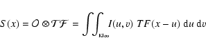$$S(x) = {\cal O} \otimes {\cal TF} = \int\!\!\int_{_{\rm Kleo}} \!\! I(u,v)\;TF(x-u)\;{\rm d}u~{\rm d}v$$ (1)

where I(u,v) is the brightness distribution, and the integral limits are given by the target's shape as obtained from the physical ephemerides (see Sect. 2). These interferograms can be computed in a straightforward manner by numerical integration for any shape modeled by polygons and vertices given in topographic coordinates.

Kleopatra was observed with the HST/FGS astrometer on January 13, 2000, providing data with a moderate to good signal-to-noise ratio (Tanga et al. 2001). Due to the limitation in time allocation, the observing run covers only 15% of Kleopatra's 5.385 hour rotation period (see Table 1). Deriving shape models from the inversion of these data is limited by such short time-span, but on the other hand, the high resolution HST/FGS data can provide valuable information and constraints on existing 3-dimensional topographic models. The HST observing run is divided into 17 visits of about 2.5 min duration each, producing a number of S-curves given by Eq. (1) along the two perpendicular FGS-X and -Y axes. The orientation of Kleopatra with respect to the FGS axes is given in Fig. 3 for the last visit. The sub-Earth point longitude was increasing from  $50\hbox{$^\circ$ }$ at the first visit, to $92\hbox{$^\circ$ }$ at the last visit.

Figure 4 shows the comparison of the radar model to the HST/FGS observations for five arbitrarily selected visits. The modeled S-curve in Eq. (1) needs to be translated both along the abscissa and ordinate directions to check the agreement with the observations. This is done by minimizing the residuals over the interval $x\in[-0.4;~0.4]$. This procedure is of little consequence, but useful to mention in order to understand the meaning of the superposition of the observed and computed curves in case of lower goodness of fit. It appears that the discrepancies between the observed and calculated data are, on the average, within the uncertainties of the nominal shape model of Kleopatra. However the residuals between the observed and calculated interferograms are larger - and statistically significant - in the second half of the observing run. These systematic features on the residuals, approximately two to three times larger than the typical rms of the FGS observational data noise, shows that the HST/FGS data available for Kleopatra can valuably constrain the shape determination of this object.

 

 

Table 1: HST/FGS observations log from January 2000, 13.

Visit #	UTC mid [hr]	Visit #	UTC mid [hr]
1	13.57	a	13.93
2	13.62	b	13.97
3	13.66	c	14.01
4	13.70	d	14.05
5	13.74	e	14.09
6	13.78	f	14.13
7	13.82	g	14.17
8	13.86	h	14.21
9	13.89

Figure 3: Physical ephemeris of the shape model for Kelopatra on the last visit.