The phase-averaged X-ray light curves of the two ROSAT and the XMM-Newton observations (summed signal from all three cameras) are shown in Fig. 1. At all occasions the source showed a pronounced on/off behavior with the eclipse roughly centered on the X-ray bright phase. The eclipse was covered 3 times in 1992, 8 times in 1993, and 2 times in the PN-observation (good time intervals only, one eclipse was excluded from the analysis due to high particle background).
In the 1992 observation the source showed a pronounced flare at phase 0.2. The end of the bright phase was not covered, the length of the bright phase, however, was inferred by RC94 from contemporaneous optical photometry. A pre-eclipse dip, likely due to the intervening accretion stream occurred centered at phase 0.94. Interestingly, this feature was never observed again, indicating a re-arrangement of the accretion geometry.
The 1993 observation covered the X-ray bright phase completely (although marginally at the start) thus allowing to measure the length of the bright phase from X-ray data alone. The source displayed similar brightness during the two ROSAT observations. The eclipse appeared centered on the bright phase.
In 2000, the shape of the X-ray bright phase appeared almost unchanged compared to the 1993 observation. The eclipse now was clearly off-centered with respect to the bright phase. The rise to the bright phase was somewhat less steep than the fall. Compared with the earlier ROSAT observations, DP Leo appeared fainter in the center of the bright phase. According to Ramsay et al. (2001) and Pandel et al. (2002) DP Leo was in a state of intermediate accretion at the time of the XMM-Newton observations, whereas it was in a high state at the time of the ROSAT observations. The comparison of published results combined with our own analysis shows that the situation might be different.
For the PSPC observations of 1992, RC94 derive a bolometric
black-body luminosity for an assumed distance of 260 pc of
![]() erg s-1. Scaling to the more likely distance of
400 pc gives
erg s-1. Scaling to the more likely distance of
400 pc gives
![]() erg s-1.
RC94 used a geometry factor
erg s-1.
RC94 used a geometry factor
![]() .
Ramsay et al. (2001) used
.
Ramsay et al. (2001) used
![]() -
-
![]() and a distance of 400 pc and derive
and a distance of 400 pc and derive
![]() erg s-1 with the EPIC MOS detectors, more than twice
that value with the EPIC PN detector (for
erg s-1 with the EPIC MOS detectors, more than twice
that value with the EPIC PN detector (for
![]() cm-2 and
cm-2 and
![]() eV).
Within the accuracy of the measurements and scaled to the same geometry
factors the luminosities of the soft components at both epochs
agree with each other.
eV).
Within the accuracy of the measurements and scaled to the same geometry
factors the luminosities of the soft components at both epochs
agree with each other.
Contrary to the PSPC observations in 1992, there is a clear
detection of DP Leo above 0.5 keV in the PSPC observation
performed in 1993, which allows fitting
of a two-component spectrum. With the spectral resolution
provided by the ROSAT PSPC, the spectrum
is well reflected by a combination of a black-body and a bremsstrahlung
component. We fixed the bremsstrahlung temperature at
the typical temperature of
![]() keV. The bolometric
flux in the bremsstrahlung component thus derived was
keV. The bolometric
flux in the bremsstrahlung component thus derived was
![]() erg cm-2 s-1.
erg cm-2 s-1.
Application of the same simple model to the EPIC PN data, and adding
a Gaussian for the iron line at 6.7 keV, gives a fitted temperature of
![]() keV and a bolometric flux of
keV and a bolometric flux of
![]() erg cm-2 s-1, which again is
not in contradiction to the former ROSAT measurements. We conclude
that the X-ray observations do not indicate an
obvious change of the mass accretion rate between the three epochs.
erg cm-2 s-1, which again is
not in contradiction to the former ROSAT measurements. We conclude
that the X-ray observations do not indicate an
obvious change of the mass accretion rate between the three epochs.
Schmidt et al. (1994) have shown that the HST-UV light curve and spectra can be understood in terms of a white-dwarf plus accretion hot spot. They fitted the spot-on and -off (i.e. white dwarf) spectra with black body models of 50 000 K and 16 000 K, respectively. Proper white-dwarf model spectra for Hydrogen atmospheres were developed by one of us (Gänsicke et al. 1995, 1998). These models were applied to the HST- and OPTIMA-data, making use of the time and spectral information in these data sets.
We firstly fitted our models to
mean faint- and bright-phase spectra (phase
intervals 1 and 2 in Fig. 5, respectively), and determined
the undisturbed white dwarf temperature to be
![]() K,
and the mean spot temperature to be
K,
and the mean spot temperature to be
![]() K. We
assumed a distance of D = 400 pc and a white dwarf radius of
K. We
assumed a distance of D = 400 pc and a white dwarf radius of
![]() cm (see Fig. 4).
cm (see Fig. 4).
Secondly, we fitted the observed light curve, both the overall shape,
i.e. the length and phasing of the bright phase with respect to the
eclipse center, as well as the detailed shape of the eclipse.
Our model assumes a circular flat accretion spot with linear temperature
decrease from a maximum
![]() in the center down to the
temperature
in the center down to the
temperature
![]() of the undisturbed atmosphere at some polar angle
of the undisturbed atmosphere at some polar angle
![]() .
Further parameters of the model are the orbital inclination i, the
co-latitude
.
Further parameters of the model are the orbital inclination i, the
co-latitude ![]() and longitude
and longitude ![]() of the accretion spot, the radius of the
white dwarf, the distance to the binary star and the time of inferior
conjunction of the secondary. We assume, that the secondary fills
its Roche lobe, that the mass-radius relation of Caillault &
Patterson (1990) applies, and that the eclipse is determined purely
by geometric parameters (and not e.g. by the atmosphere of the
secondary).
The parameters were
varied until a sufficient fit with the observations was reached.
of the accretion spot, the radius of the
white dwarf, the distance to the binary star and the time of inferior
conjunction of the secondary. We assume, that the secondary fills
its Roche lobe, that the mass-radius relation of Caillault &
Patterson (1990) applies, and that the eclipse is determined purely
by geometric parameters (and not e.g. by the atmosphere of the
secondary).
The parameters were
varied until a sufficient fit with the observations was reached.
In these model calculations,
the radius of the white dwarf
![]() can be traded against the distance,
as far as the overall brightness of the system is concerned.
We therefore explored two cases of a white dwarf, a standard white
dwarf with 0.6
can be traded against the distance,
as far as the overall brightness of the system is concerned.
We therefore explored two cases of a white dwarf, a standard white
dwarf with 0.6 ![]() and a massive white dwarf with 1
and a massive white dwarf with 1 ![]() ,
as
proposed recently by Ramsey et al. (2000). In order to reproduce the
observed light curve, one has to assume
significantly different sizes and temperatures of the accretion
spot for the two cases. These result in distinct
differences at eclipse ingress and egress, which allows
to discern between the two models.
Satisfactory agreement between observation and model were reached
for the following set of parameters:
,
as
proposed recently by Ramsey et al. (2000). In order to reproduce the
observed light curve, one has to assume
significantly different sizes and temperatures of the accretion
spot for the two cases. These result in distinct
differences at eclipse ingress and egress, which allows
to discern between the two models.
Satisfactory agreement between observation and model were reached
for the following set of parameters:
![]()
![]() ,
,
![]() ,
,
![]() ,
,
![]() ,
,
![]() ,
,
![]() ,
,
![]() K,
K,
![]() K. The time of inferior conjunction of the
secondary according to this fit is listed in Table 2.
Uncertainties of the parameters were estimated from eyeball inspection
of the light curve fits. Our best-fit light curve is shown in
Fig. 5.
K. The time of inferior conjunction of the
secondary according to this fit is listed in Table 2.
Uncertainties of the parameters were estimated from eyeball inspection
of the light curve fits. Our best-fit light curve is shown in
Fig. 5.
![\begin{figure}
\par\includegraphics[width=8.8cm,clip]{dpleo_bg1.ps}\end{figure}](/articles/aa/full/2002/35/aah3063/img77.gif) |
Figure 4:
HST/FOS spectra averaged over the phase interval labelled 1 and 2
in Fig. 5.
The Ly
|
![\begin{figure}
\par\includegraphics[angle=-90,width=17cm,clip]{hst_eclfit.ps}\end{figure}](/articles/aa/full/2002/35/aah3063/img78.gif) |
Figure 5: Fit to the HST/FOS light curve with a model containing an eclipsed white dwarf and a flat circular accretion spot on it. The temperature falls linearly from a maximum in the center to the undisturbed white dwarf atmosphere. Fit parameters and best-fit values are described in Sect. 3.2. Numbers "1'' and "2'' in the lower panel indicate those phase intervals which were used for the spectral fit shown in Fig. 4. |
The OPTIMA light curve shown in Fig. 3
looks different than those of the FOS or
other optical eclipse light curves published previously
(e.g. Bailey et al. 1993).
After the initial steep ingress into eclipse
a distinct source of radiation is still present.
This light curve looks similar to those of UZ For (Kube et al. 2000)
or HU Aqr (Schwope et al. 1993) and the remaining emission
is clearly due to the accretion
stream which is still visible after eclipse of the white dwarf.
The stream was not seen in earlier eclipse
light curves of DP Leo, hence a distinct rearrangement of the
accretion geometry has taken place.
For our analysis of the eclipse of the white dwarf the stream
is a contaminating source and we subtract it by approximating its
contribution by a low-order
polynomial (dotted line in Fig. 3).
The residua are fitted by the same model as it was applied to the HST-data.
We cannot, however, re-determine the temperature of the white dwarf
and/or the spot, since a mixture of different radiation
components of different origin is present in the optical.
The optical light
curve has a photospheric component, radiation from the accretion spot
and cyclotron radiation from the accretion shock, which cannot be uniquely
disentangled without spectral or multiband photometric information.
The model is nevertheless useful in order to re-determine
the size of the emission region(s) and to determine the time
of superior conjunction of the white dwarf. Our best-fit, shown
in Fig. 6, implies a somewhat smaller accretion spot,
![]() ,
than present in the HST-data.
The time of inferior conjunction of the
secondary is also listed in Table 2. According to the most
likely position of the accretion spot as derived from X-ray observations,
the azimuth of the accretion spot was fixed at 27
,
than present in the HST-data.
The time of inferior conjunction of the
secondary is also listed in Table 2. According to the most
likely position of the accretion spot as derived from X-ray observations,
the azimuth of the accretion spot was fixed at 27![]() during the
fitting process. The eclipse
of the accretion spot, which causes the steep part of the eclipse light curve,
therefore appears slightly offcentered
from true phase zero and the whole light curve appears asymmetric.
during the
fitting process. The eclipse
of the accretion spot, which causes the steep part of the eclipse light curve,
therefore appears slightly offcentered
from true phase zero and the whole light curve appears asymmetric.
Application of our method to the X-ray data of DP Leo allowed an accurate determination of the eclipse length at X-ray wavelengths. The measurements at all three epochs agree with each other within the claimed accuracy, ranging from 233 s to 237 s with a 5 s accuracy (see Table 1).
The new determination of the eclipse length has a much higher accuracy
than that by RC94, who give ![]() s.
RC94 derive an upper limit of
s.
RC94 derive an upper limit of ![]() 22 s on the length of the
eclipse ingress/egress phase.
The binned eclipse light curves of Fig. 2
clearly show, that eclipse ingress and egress lasts much shorter
than 22 s in the observations perfomed in 1993 and 2000
but the count rate is not sufficient to resolve ingress and egress.
We therefore cannot derive strong
constraints on the lateral extent of the X-ray emission
region. For comparison, in UZ For and HU Aqr where the egress phases
could be resolved by EUVE and ROSAT observations, respectively,
these features last only about 1.3 s (Warren et al. 1995;
Schwope et al. 2001), corresponding to a full opening angle of the
X-ray emission region on the white dwarf of only 3
22 s on the length of the
eclipse ingress/egress phase.
The binned eclipse light curves of Fig. 2
clearly show, that eclipse ingress and egress lasts much shorter
than 22 s in the observations perfomed in 1993 and 2000
but the count rate is not sufficient to resolve ingress and egress.
We therefore cannot derive strong
constraints on the lateral extent of the X-ray emission
region. For comparison, in UZ For and HU Aqr where the egress phases
could be resolved by EUVE and ROSAT observations, respectively,
these features last only about 1.3 s (Warren et al. 1995;
Schwope et al. 2001), corresponding to a full opening angle of the
X-ray emission region on the white dwarf of only 3![]() .
.
![\begin{figure}
\par\includegraphics[angle=-90,width=18cm,clip]{opt_eclfit.ps}\end{figure}](/articles/aa/full/2002/35/aah3063/img81.gif) |
Figure 6: Fit to the OPTIMA light curve after correction for residual emission from the accretion stream as shown with a dotted line in Fig. 3. The model is the same as used for the HST-data, although an absolute calibration was not possible for the white-light OPTIMA bandpass. Best-fit values are given in Sect. 3.3. |
| (1) | (2) | (3) | (4) | (5) | (6) |
| Epoch | Cycle | BJED | Type(1) | ||
| -2 400 000 | (s) | (s) | |||
| 1979.9 | -73 099 | 44214.55325 | 15 | +5.7 | X |
| 1979.9 | -73 098 | 44214.61562 | 15 | +5.7 | X |
| 1979.9 | -73 097 | 44214.67798 | 15 | +5.7 | X |
| 1982.0 | -61 017 | 44968.02309 | 100 | -- | O |
| 1982.0 | -61 002 | 44968.95712 | 100 | -- | O |
| 1982.0 | -61 001 | 44969.01962 | 100 | -- | O |
| 1982.0 | -60 841 | 44978.99755 | 100 | -- | O |
| 1982.1 | -60 602 | 44993.90078 | 60 | -- | O |
| 1982.1 | -60 601 | 44993.96328 | 60 | -- | O |
| 1982.1 | -60 600 | 44994.02642 | 60 | -- | O |
| 1982.1 | -60 169 | 45020.90513 | 20 | -- | O |
| 1982.1 | -60 153 | 45021.90292 | 20 | -- | O |
| 1982.2 | -60 106 | 45024.83386 | 60 | -- | O |
| 1984.1 | -48 767 | 45731.96640 | 30 | -- | O |
| 1984.2 | -48 256 | 45763.83373 | 5 | -- | O |
| 1984.4 | -46 796 | 45854.88280 | 100 | -- | X |
| 1985.0 | -43 588 | 46054.94231 | 100 | -- | X |
| 1985.1 | -43 075 | 46086.93565 | 3 | -- | O |
| 1985.1 | -43 074 | 46086.99796 | 3 | -- | O |
| 1991.8 | -3410 | 48560.55780 | 4 | 0.0 | UV |
| 1992.4 | 0 | 48773.21509 | 5 | -0.5 | X |
| 1992.4 | 16 | 48774.21293 | 5 | -0.5 | X |
| 1993.4 | 5848 | 49137.91294 | 5 | -1.2 | X |
| 1993.4 | 5945 | 49143.96214 | 5 | -1.2 | X |
| 1993.4 | 5946 | 49144.02438 | 5 | -1.2 | X |
| 1993.4 | 5947 | 49144.08689 | 5 | -1.2 | X |
| 1993.4 | 5961 | 49144.96005 | 5 | -1.2 | X |
| 1993.4 | 5962 | 49145.02235 | 5 | -1.2 | X |
| 1993.4 | 5963 | 49145.08454 | 5 | -1.2 | X |
| 1993.4 | 5964 | 49145.14711 | 5 | -1.2 | X |
| 2000.9 | 49 670 | 51870.77688 | 5 | -6.2 | X |
| 2000.9 | 49 672 | 51870.90163 | 5 | -6.2 | X |
| 2002.0 | 56 307 | 52284.67895 | 5 | 0.0 | O |
We update the eclipse ephemeris of DP Leo by using X-ray data combined with HST- and OPTIMA observations.
For the determination of the combined optical/UV/X-ray
eclipse ephemeris, the times
of the measured eclipse centers at X-ray wavelengths
were corrected for the small phase offset
between eclipse of the spot and eclipse of the white dwarf using the
values as given in Table 2.
These numbers are based on the following parameters of the binary:
![]() ,
mass-radius relations for the white dwarf and the secondary by
Nauenberg (1972) and Caillault & Patterson (1990),
spot latitude 100
,
mass-radius relations for the white dwarf and the secondary by
Nauenberg (1972) and Caillault & Patterson (1990),
spot latitude 100![]() ,
spot longitude as given in Table 1
(the longitude at the time of the EINSTEIN observation was -22
,
spot longitude as given in Table 1
(the longitude at the time of the EINSTEIN observation was -22![]() ).
Usage of these parameters gives the correct eclipse length and length
of the bright phase, if a height of the emission region of 0.02
).
Usage of these parameters gives the correct eclipse length and length
of the bright phase, if a height of the emission region of 0.02
![]() is taken into account. The assumed height is in accord with other
polars (e.g. Schwope et al. 2001).
The small corrections to the eclipse times as listed in the above
table are
+5.7, -0.5, -1.2, -6.2 s for the EINSTEIN, ROSAT 1992,
ROSAT 1993, and the XMM-Newton observations, respectively.
is taken into account. The assumed height is in accord with other
polars (e.g. Schwope et al. 2001).
The small corrections to the eclipse times as listed in the above
table are
+5.7, -0.5, -1.2, -6.2 s for the EINSTEIN, ROSAT 1992,
ROSAT 1993, and the XMM-Newton observations, respectively.
A linear regression to the corrected X-ray eclipse times together
with the HST and OPTIMA measurements
does not give a satisfactory fit to the data.
The fit is good after inclusion of a quadratic term.
Our finally adopted ephemeris is
![\begin{figure}
\par\includegraphics[angle=-90,width=8.8cm,clip]{omc_quad.ps}\end{figure}](/articles/aa/full/2002/35/aah3063/img89.gif) |
Figure 7: Plot of the X-ray, UV and OPTIMA eclipse times of the white dwarf's center of mass after subtraction of the linear trend. At X-ray wavelengths the originally measured quantity which corresponds to the time of eclipse of the accretion spot was corrected to center of mass using the values given in the fifth column of Table 2. At optical/UV wavelengths the time of mid-eclipse of the white dwarf was determined by the fitting procedure described in the text (Sects. 3.2 and 3.3). Crosses indicate X-ray data, circles indicate HST- and OPTIMA-data. The dotted curve is the finally accepted ephemeris of the white dwarf's superior conjunction. |
The large shift of the bright phase with respect to the eclipse
is interesting as such. RC94 noticed that since the early
observations in 1980 the bright phase was continuously shifted
from negative longitudes to about zero longitude in 1992 and they
deduced a yearly shift of the spot longitude of 2.05![]() .
The data collected in Table 1 imply that this
shift might become even larger,
.
The data collected in Table 1 imply that this
shift might become even larger,
![]() yr-1.
Figure 8 shows the synopsis of all the bright phase
center (spot longitude) measurements. The phase shift is continuous
and monotonic over the last 20 years. The spot started at negative
longitudes, i.e. in the half-sphere away from the ballistic
accretion stream and now approaches the more typical (natural?)
location at about 30
yr-1.
Figure 8 shows the synopsis of all the bright phase
center (spot longitude) measurements. The phase shift is continuous
and monotonic over the last 20 years. The spot started at negative
longitudes, i.e. in the half-sphere away from the ballistic
accretion stream and now approaches the more typical (natural?)
location at about 30![]() (see Cropper 1988, for a compilation of
accretion spot longitudes).
(see Cropper 1988, for a compilation of
accretion spot longitudes).
Spot longitude variations can be caused by changes of the mass accretion rate, by synchronization oscillations or by an asynchronously rotating white dwarf. Accretion rate changes would not imply a monotonic phase shift, they would imply a positive spot longitude at high accretion rate and a smaller longitude at low accretion rate. Since the accretion rate most probably did not change considerable between the ROSAT and the XMM-Newton observations, spot longitude are difficult to explain this way.
Synchronization oscillations are predicted to occur
once a locked state between the white
dwarf and the secondary star is reached (Campbell 1989; King & Whitehurst 1991).
So far no measurement
could be performed in order to test the theory, the relevant
time-scales and the amplitudes of these oscillations.
The predicted period of small oscillations about the locked state
is
![]() yr (Campbell & Schwope 1999),
i.e. of the order of the time base
covered meanwhile by the observations.
There is no indication of a
reversal of the spot longitude migration implied by an oscillation
scenario. We therefore tend to favor the scenario of a dis-locked white
dwarf and thus add DP Leo to the small sub-class of asynchronous
polars with so far four members only (Campbell & Schwope 1999).
If our assignment is correct,
DP Leo is different from the other systems in this sub-class
showing a much smaller
degree of asynchronism. RC94 already estimated the deviation
yr (Campbell & Schwope 1999),
i.e. of the order of the time base
covered meanwhile by the observations.
There is no indication of a
reversal of the spot longitude migration implied by an oscillation
scenario. We therefore tend to favor the scenario of a dis-locked white
dwarf and thus add DP Leo to the small sub-class of asynchronous
polars with so far four members only (Campbell & Schwope 1999).
If our assignment is correct,
DP Leo is different from the other systems in this sub-class
showing a much smaller
degree of asynchronism. RC94 already estimated the deviation
![]() ,
whereas
the absolute of this quantity in the other four is
,
whereas
the absolute of this quantity in the other four is ![]() 10-2.
We note that we cannot properly measure the spin period of the white
dwarf in DP Leo, since the accretion spot is not fixed in the magnetic
coordinate system of the white dwarf.
Should the degree of asynchronism be of the order as derived here,
a fundamental re-arrangement of the accretion geomtry
in terms of a pole-switch must occur
sometimes in the not too far future.
10-2.
We note that we cannot properly measure the spin period of the white
dwarf in DP Leo, since the accretion spot is not fixed in the magnetic
coordinate system of the white dwarf.
Should the degree of asynchronism be of the order as derived here,
a fundamental re-arrangement of the accretion geomtry
in terms of a pole-switch must occur
sometimes in the not too far future.
We searched the XMM-Newton data for photons in the eclipse, which would be ascribed to the putative active secondary star. Omitting the first and last 10 s of the eclipse the total exposure time in eclipse investigated by us was 1436 s and included 6 eclipses (three cameras) in good time intervals. In the source-plus-background region 29 photons were registered, while in the neighboring background region only 18 photons were registered.
In order to estimate the likely count rate only from the source, we employed a Bayesian estimate using a method described by Loredo (1992), which is applicable to a dataset with low number of counts having a Poisson distribution.
The most probable value of the count rate was 0.0075 cts s-1 taken from
the evaluated full Bayesian probability distribution function. A Bayesian
credible region (a "posterior bubble'')
is 0.0030-0.0120 cts s-1 in a 68% (1![]() )
confidence interval.
The 99.73% (3
)
confidence interval.
The 99.73% (3![]() )
credible region gives a value 0.0000-0.0212 cts s-1,
consistent with zero. We regard our finding as uncertain marginal
detection of the secondary in X-rays.
)
credible region gives a value 0.0000-0.0212 cts s-1,
consistent with zero. We regard our finding as uncertain marginal
detection of the secondary in X-rays.
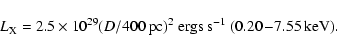
With the nominal count rate the luminosity of the secondary is
This estimate is consistent with coronal emission of late type stars from the solar vicinity (Hünsch et al. 1999).
Copyright ESO 2002
![\begin{figure}
\par\includegraphics[angle=-90,width=8.8cm,clip]{longi_shift.ps}\end{figure}](/articles/aa/full/2002/35/aah3063/img90.gif)