A&A 391, 809-821 (2002)
DOI: 10.1051/0004-6361:20020588

Distributions, equivalent widths and metallicities of the H II regions in the spiral galaxies NGC 5457
and NGC 4395

B. Cedrés¹ - J. Cepa^1,2

1 - Instituto de Astrofísica de Canarias, 38205 La Laguna, Tenerife, Spain
2 - Departamento de Astrofísica, Facultad de Física, Universidad de La Laguna, 38071 La Laguna, Tenerife, Spain

Received 19 November 2001 / Accepted 16 April 2002

Abstract
Using CCD observations in the narrow band filters in H$\alpha$, H$\beta$, [O II], [O III], [S II] and [S III] lines we have compiled a catalogue of 338 H II regions for the inner parts of NGC 5457 and 158 for NGC 4395. The extinction, equivalent widths, distributions, excitations, ionization hardness, ionization parameters and metallicities for these regions, a distinction being made between arm and inter-arm zones, are presented here with the first results of a study of stellar formation.

Key words: H II regions - galaxies: individual: NGC 4395, NGC 5194 - galaxies: abundances

1 Introduction

As part of a work to evaluate the differences in the stellar formation occurring in the arm and inter-arm regions of grand design galaxies and to compare this type of star formation with that in flocculent galaxies, we have obtained images using narrow band filters for the wavelengths H$\alpha$, H$\beta$, [O II] $_{\lambda\lambda3726,~3729}$, [O III] $_{\lambda5007}$, [S II] $_{\lambda\lambda6717,~6731}$ and [S III] $_{\lambda9069}$ and their respective continua. We present here the distribution, extinctions, equivalent widths, excitations, ionization hardness, ionization parameters and metallicities of the H II regions observed.

For this study we have selected NGC 5457 (a grand design spiral galaxy) and NGC 4395 (a flocculent spiral galaxy). NGC 5457 is a type 9 galaxy (from Elmegreen & Elmegreen 1987, classification). It has been previously studied (together with other galaxies) by Searle (1971) and Smith (1975), who established the existence of metallicity gradients in discs. Other spectrophotometric observations have been carried out by van Zee et al. (1998), Kennicutt & Garnett (1996), Scowen et al. (1992) and others cited by these workers. NGC 5457 has been studied in the X-ray regime by Williams & Chu (1995), who discovered that several of the detected sources were giant H II regions and explained this emission as a mixture of X-ray binaries and supernova remnants (SNRs). This galaxy was selected due its size and number of bright H II regions.

NGC 4395 is a type 1 galaxy (Elmegreen & Elmegreen 1987) and is the complete opposite to NGC 5457 in terms of its properties. It has chaotic, fragmented and asymmetric arms, but hosts intense star formation processes, with bright H II regions.

NGC 4395 has been studied in detail by Roy et al. (1996), who have discovered that there is no global O/H abundance gradient across the disc. They explained this in terms of a large scale redistribution of interstellar matter over a timescale of a few galactic rotations. However, van Zee et al. (1998), taking into account new spectroscopic results, suggest there is a shallow gradient. These authors also confirm that the nucleus of this galaxy harbours a dwarf Seyfert, as was claimed by Ho et al. (1995).

All the previous works have been limited by the low number of regions (i.e. Kennicutt & Garnett 1996) because of either the spectroscopic technique or the few lines studied (i.e. Roy et al. 1996 or Scowen et al. 1992) by direct imaging. In this paper we aim to complete these earlier studies by observing a significant number of H II regions in several emission lines in order to be able to extract statistical conclusions about the star formation trends that occur in spiral galaxies.

2 Observations and data reduction

The observations were carried out during three different runs. The first was during 1999 March 19-22 at the Nordic Optical Telescope (NOT), wher we obtained the H$\alpha$, H$\beta$, [O II] and [O III] images and their continua. We used the ALFOSC instrument in direct imaging mode, with a 2 k Loral CCD (2048 $\times$ 2048 pixels) and with a scale of 0.189 $^{\prime\prime}$/pix.

The second run was during 1999 March 21-24 on the 2.2 m telescope located at Calar Alto Observatory, where we obtained the [S II] images and its continua. We used CAFOS in direct imaging mode, with an SITe#1 d CCD ( $2048~\times$2048 pixels), with a scale of 0.4996 $^{\prime\prime}$/pix.

In the last run, 2000 July 5-7, on the Calar Alto 3.5 m telescope, we obtained [S III] images and continua for NGC 5457. We used MOSCA in direct imaging mode, with an SITe-16a CCD (4096 $\times$ 4096 pixels) with a scale of 0.32 $^{\prime\prime}$/pix.

Table 1 summarizes the main parameters of the observed galaxies.

 

 

Table 1: Galaxy parameters.

Galaxy	Morphological	Arm	R25	V	i	PA
	type	class	'	km s-1	$^{\circ}$	$^{\circ}$
	(1)	(2)	(3)	(4)	(3)	(3)
NGC 4395	SA(s)m	1	6.58	318	18	147
NGC 5457	SAB(rs)cd	9	14.41	241	18	37

(1) De Vaucouleurs et al. (1991).
(2) Elmegreen & Elmegreen (1987).
(3) van Zee et al. (1998).
(4) http://nedwww.ipac.caltech.edu/

Table 2 shows the filters used and the exposure times. The first column lists the name of the filter, the second column states the central wavelength for each filter in ångströms, the third column states the full width half medium in ångströms and the last columns indicates the exposure time employed for each filter.

 

 

Table 2: Filters used and exposure times. The first column gives the name of the filter, the second column gives the central wavelength of each filter in ångströms, the third column gives the FWHM of each filter and the last column gives the exposure time employed.

Filter	$\lambda_{\rm c}$ (Å)	FWHM (Å)	Exp. time (s)
[O II] cont.	3500	330	1800
[O II]	3725	29	$3\times1800$
H$\beta$ cont.	4685	170	1800
H$\beta$	4864	26	$2\times1800$
[O III]	5012	30	$3\times1800$
[O III] cont.	5470	220	1800
H$\alpha$	6571	47	1800
H$\alpha$ cont.	6803	50	1800
[S II]	6737	66	$4\times1800$
[S II] cont.	7157	140	$2\times1800$
[S III] cont.	8510	105	$3\times1800$ (1)
[S III]	9150	350	$5\times1800$ (1)

$\parbox{7cm}{ (1) For NGC~5457 only.}$

The reduction and calibration of the data were carried out using the IRAF package. The reduction consists in bias correction using bias images (taken at the beginning of each night) and overscan zones in each image; flatfield correction using from 3 to 6 sky flats per filter taken every night of observation; sky subtraction using 21 $\times$ 21 pixel boxes in image zones not affected by the galaxy, cosmic rays or field stars; and cosmic ray elimination using the IRAF COSMICRAYS task when we only have one or two images per filter, or combining and extracting the median image when we have more than two images. With this last method we also get a better signal to noise for the resultant image.

To calibrate the data we used Oke & Gunn's (1983) and Oke's (1990) spectrophotometric standards. The calibration was carried out following Barth et al. (1994).

To subtract the continuum, all the continuum images were multiplied by factors close to unity. These factors were determined assuming that the inter-arm emission was null after the subtraction. This is preferred to the field star method, because these stars may present different spectral energy distributions from that of the stellar population of the galaxy, and also they may present strong absorption lines, so the correction factors will be underestimated or overestimated. Moreover, using this method we are able to correct every line for diffuse background emission.

To separate arm and inter-arm regions in the grand design galaxy (NGC 5457), we used broad band images in the Johnson Ifilter. We fitted a surface for inter-arm zones and then we subtracted it from the galaxy image. In this way, only the arm zones remained with positive values. With this new image we can trace the arms of the galaxy and distinguish with a very high level of confidence if an H II region belongs to the arm or to the inter-arm. Figure 1 shows the location of the arms in NGC 5457. The filled dots are the detected arm regions, open circles are the inter-arm regions.

	Figure 1: Deprojected arms for NGC 5457. Filled dots are arm regions. Open circles are inter-arm regions. Continuum lines mark the limits of the arms. The radius is expressed in arcmin.
Open with DEXTER

In Fig. 2 we show the detected regions for the northern and southern parts of NGC 5457 in H$\alpha$ (continuum-substracted). From Figs. 3 to 7 we show the obtained emission line images for NGC 5457 in H$\beta$, [O II], [O III], [S II] and [S III] respectively (all continuum-substracted). In Fig. 8 we show the detected regions for NGC 4395 in H$\alpha$ continuum-substracted. From Figs. 9 to 12 we show the emission line images for NGC 4395 in H$\beta$, [O II], [O III] and [S II] respectively (all continuum-substracted).

	Figure 2: NGC 5457 H$\alpha$ image, continuum substracted. Green dots are the detected regions.
Open with DEXTER

	Figure 3: NGC 5457 H$\beta$ image, continuum substracted.
Open with DEXTER

	Figure 4: NGC 5457 [O II] image, continuum substracted.
Open with DEXTER

	Figure 5: NGC 5457 [O III] image, continuum substracted.
Open with DEXTER

	Figure 6: NGC 5457 [S II] image, continuum substracted.
Open with DEXTER

	Figure 7: NGC 5457 [S III] image, continuum substracted.
Open with DEXTER

	Figure 8: NGC 4395 H$\alpha$ image, continuum substracted. Green dots are the detected regions.
Open with DEXTER

	Figure 9: NGC 4395 H$\beta$ image, continuum substracted.
Open with DEXTER

	Figure 10: NGC 4395 [O II] image, continuum substracted.
Open with DEXTER

	Figure 11: NGC 4395 [O III] image, continuum substracted.
Open with DEXTER

	Figure 12: NGC 4395 [S II] image, continuum substracted.
Open with DEXTER

In Figs. 13 and 14 we show the position and relative sizes for the regions detected in NGC 5457 and NGC 4395, respectively.

	Figure 13: Deprojected position of the H II regions for NGC 5457. Each circle represents a H II region with the size proportional to the region area. Radius is expressed in arcmin. Angles measured counterclockwise from the west.
Open with DEXTER

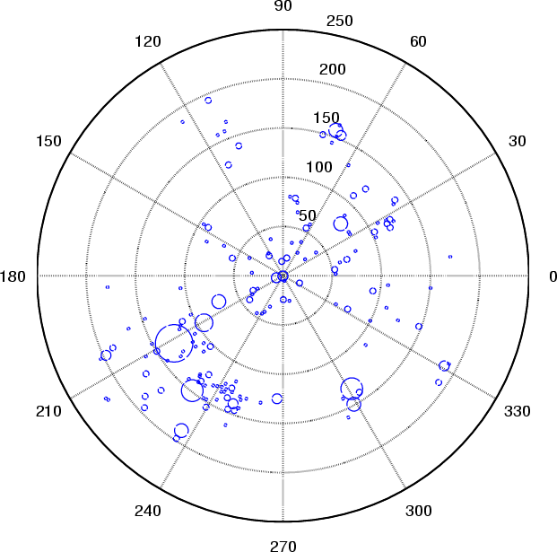	Figure 14: Deprojected position of the H II regions for NGC 4395. Each circle represents a H II region with the size proportional to the region area. Radius is expressed in arcmin. Angles measured counterclockwise from the west.
Open with DEXTER

To correct for the effect of galactic and extragalactic extinction we used a method based on the H$\alpha$ and H$\beta$rate, assuming the B case with an electronic density of 100 cm^-3 and 10 000 K (James & Puxley 1993). We also used the extinction law given by Seaton (1979),

$$A_V=2.5\ln\frac{(F_{{\rm H}\alpha}/F_{{\rm H}\beta})_{\rm observed}}{2.86}\cdot$$ (1)

Using Eq. (1) and the reddening law given by Schild (1977), we obtained the extinction for all the lines.

The underlying absorption due massive stars in H II regions could be an important source of errors when fluxes are calculated. It is possible to obtain reductions on H$\beta$ equivalent widths of about 50% (McCall et al. 1985), which leads to overestimation of the absorption. To correct for this effect, we use the method defined by McCall et al. (1985), which allows us to correct for the underlying absorption effect using the equivalent widths of the H$\alpha$ and H$\beta$lines. Since the internal (non-atmospheric) extinction is different in the line and the continuum due to the different central wavelengths of the filters used, it is necessary to apply an iterative process to correct for underlying absorption and to derive extinctions: initially the H$\alpha$ and H$\beta$ equivalent widths uncorrected for extinction are calculated. From these we evaluate the absorption-corrected H$\beta$ fluxes before deriving the internal extinction. This internal extinction is used to correct the H$\alpha$ and H$\beta$ line and continuum fluxes. Using these first order extinction-corrected fluxes, we calculate the equivalent widths again, and the H$\beta$ flux is later corrected for underlying absorption, which allows the determination of the extinction, etc. This procedure is repeated until convergence is obtained, which takes only few iterations.

Due to H$\alpha$ width the H$\alpha$ fluxes are contaminated by the [NII] $\lambda\lambda$6548, 6584 lines. To correct for this effect we used the data given by McCall et al. (1985) assuming a linear gradient for the behaviour of [NII]/H$\alpha$.

The continuum H$\alpha$ and H$\beta$ fluxes of H II regions were also contaminated by the emission from the underlying galactic disc. To avoid this effect, we applied a box median filter to the continuum image. We selected the size of the box wider enough to avoid sampling the H II regions but narrower than the arms size to sample them. With this process we obtained an image of the galactic disk, including the arms. After this, we substracted this image from the continuum image and then we calculated the extinctions and equivalent widths.

The fluxes were extracted using the FOCAS task. With this program we created limiting isophotes for each region defined where the flux for the region was under 3$\sigma$ of the background. After that, we created a mask for each region using this isophote as the limiting border, and we multiplied this mask for the line image, getting the emission flux for this new image easily using only the IRAF IMSTATISTICS task.

3 Results

  
3.1 The data

Tables 3 to 5 present the data obtained for NGC 5457, and Tables 6 to 8 present the data for NGC 4395 .

Table 3 summarizes the properties of the H II region sample for NGC 5457. Column 1 is the region identification number. Columns 2 and 3 are the position of the region in the galaxy, in arcsec, with respect to the nucleus with east and north positive. Column 4 lists the deprojected galactocentric radius, R, in arcminutes, assuming an inclination of 18$^{\circ}$ and a position angle of 37$^{\circ}$ (van Zee et al. 1998). Column 5 lists the visual extinction in magnitudes for each region. Column 6 lists the extinction-corrected H$\alpha$ flux in units of 10^-13 erg cm^-2 s^-1. Column 7 lists the base 10 logarithm of H$\alpha$ equivalent width, with the equivalent width expressed in Å. Column 8 lists the extinction corrected H$\beta$ flux in units of 10^-13 erg cm^-2 s^-1. Column 9 lists the base 10 logarithm of H$\beta$ equivalent width, with the equivalent width expressed in Å. Column 10 indicates whether the region belongs to the arm (A) or interarm (I) zones. Table 6 summarizes the properties of the H II regions for NGC 4395. The distribution of the columns are the same as for Table 3, but without Col. 10.

Table 4 summarizes the flux for several emission lines for NGC 5457. Column 1 lists the identification number of the region. Columns 2-5 list the [O II], [O III], [S II] and [S III] ratios. All the quantities are relative to H$\beta=100$ and extinction corrected. We have assumed the theoretical relations: I([O III] $\lambda\lambda4959,5007$) = 1.34I([O III] $\lambda5007$) and I([S III] $\lambda\lambda9069,9532$) = 3.43I([S III] $\lambda9069$).

Table 7 gives the same as Table 4 but for NGC 4395. In this case, there is no Col. 5 because we did not obtain [S III] images for this galaxy.

In Table 5 we summarize several quatities derived for line ratios for NGC 5457. Column 1 is the region identification number, Col. 2 is the R₂₃ parameter defined in Eq. (2),

$${R}_{23}=\frac{I([\mbox{\rm O\,{\sc ii}}]\lambda3727)+I([\mbo... ...O\,{\sc iii}}]\lambda\lambda4959,5007)}{I({\rm H}\beta)} \cdot$$ (2)

This parameter was introduced by Pagel et al. (1979) as an empirical oxygen abundance indicator when the temperature-sensitive lines such as [O III]$\lambda$4363 are unavaliable.

Column 3 is the oxygen abundance derived from Zaritsky et al.'s (1994) calibration, defined in Eq. (3),

 

$$12+\log(\rm {O}/\rm {H})=9.265-0.33x-0.202x^{2} -0.207x^3-0.333x^4,$$ (3)

where $x = \log R_{23}$.
Column 4 is the $\eta ^{\prime }$ parameter defined in Eq. (4).

$$\eta^{\prime}=\frac{[\mbox{O\,{\sc ii}}]\lambda\lambda3726,29... ...mbda6717,31/[\mbox{S\,{\sc iii}}]\lambda\lambda9069,9532}\cdot$$ (4)

This parameter is the observable quatitiy of the ionization hardness parameter, defined by Vílchez & Pagel (1988),

$$\eta=\rm\frac{O^+/O^{++}}{S^+/S^{++}}$$ (5)

that can be write in the following terms,

$$\log \eta=\log \eta^{\prime}+\frac{0.14}{t}+0.16$$ (6)

where $t=T_{\rm e}/10^4$, and it is assumed the low-density limit and no temperature fluctuations.

Table 8 summarizes the same as Table 5 but for NGC 4395. In this case there is no Col. 4.

3.2 Extinction

To obtain the values for the extinction, we employed the relation given in Eq. (1).

Figure 15 shows the number of region with different extinction using a histogram for NGC 5457. Figure 16 shows the extinction also but for arm (upper panel) and inter-arm (bottom panel) regions. We obtained a mean value of A_V=0.79 for all the regions and 0.71 for arm and 0.91 for inter-arm regions.

	Figure 15: Histogram for extinction in NGC 5457.
Open with DEXTER

	Figure 16: Histogram for extinction in NGC 5457. Top panel, arm regions; down panel inter-arm regions.
Open with DEXTER

Figure 17 shows the numbers of regions with different extinction for NGC 4395.

There is a clear difference in extinction between the flocculent galaxy and the grand design galaxy. For the flocculent one there are many regions with values for extinction equal to or close to 0, whereas for NGC 5457 the mean is closer to 1 and is distributed in a somewhat Gaussian style.

	Figure 17: Histogram for extinction in NGC 4397.
Open with DEXTER

3.3 Equivalent widths

The H$\alpha$ equivalent width provides a measure of the ratio of ionizing photons from massive stars and continuum photons from the embedded stars and gas. Therefore, it is sensitive to variations in the initial mass function (IMF), the stage of evolution of ionizing stars and the metallicity (Leitherer et al. 1999; Kennicutt et al. 1989; Martin & Friedli 1999; Bresolin & Kennicutt 1997). Generally, the EW(H$\alpha$) in disc galaxies goes from 100 Å to 1500 Å, with a mean value of 400 Å.

3.3.1 Equivalent widths for NGC 5457

In Fig. 18 we show the histogram for the logarithm of H$\alpha$ equivalent width for NGC 5457. The mean value for this galaxy is $\log$ ( $EW\rm [H\alpha])=3.22$, which is equivalent to an age of between 1.6 and 4 Myr, depending on the IMF selected (using Leitherer et al. 1999 models).

	Figure 18: Histogram for log of H$\alpha$ equivalent width in NGC 5457.
Open with DEXTER

Figure 19 shows the H$\alpha$ equivalent width for the arm zones (upper panel) and for the inter-arm zones (lower panel). The arm zones and inter-arm zones too yield a mean value of $\log~(EW[\rm H\alpha])=3.22$.

	Figure 19: Histogram for log of H$\alpha$ equivalent width in NGC 5457. Top panel, arm regions; down panel inter-arm regions.
Open with DEXTER

In Fig. 20 we show the H$\alpha$ equivalent width as a function of galactocentric radius for NGC 5457. Filled dots are arm regions, open circles are inter-arm regions.

	Figure 20: H$\alpha$ equivalent width as a function of galactocentric radius for NGC 5457. Filled dots are arm regions, open circles are inter-arm regions.
Open with DEXTER

The general trend is an almost constant value for the equivalent width with the radius, which indicates that the continuum diffuse emission form the disk was successfully removed. Figure 20 clearly indicates that arm and inter-arm regions present, in general, simillar values for equivalent width.

3.3.2 Equivalent widths for NGC 4395

Figure 21 shows the H$\alpha$ equivalent width for NGC 4395. We obtain a mean value of log $(EW[\rm H\alpha])=2.99$, which is equivalent ot an age of 4 Myr.

Figure 22 shows the H$\alpha$ equivalent width as a function of galactocentric radius for NGC 4395. Although for this galaxy we have less regions, the distribution is somewhat simillar to NGC 5457 with no clear tendence with the radius.

	Figure 21: Histogram for log of H$\alpha$ equivalent width in NGC 4395.
Open with DEXTER

	Figure 22: H$\alpha$ equivalent width as a function of galactocentric radius for NGC 4395.
Open with DEXTER

3.4 Line ratios and excitation

The H II regions can be categorized as "high excitation'' or "low excitation'' in terms of large or small values of the ratio [O III]/H $\beta=I(\lambda\lambda$5007, 4959)/I($\lambda$4861) (Aller 1942; Searle 1971). Empirically, strong [O III] lines are related with low oxygen abundance, high gas temperature and a large value in < $X(\rm O^{+2})$>, where <X> is a nebular average (Searle 1971; Smith 1975; Shields 1990).

3.4.1 Excitation for NGC 5457

Figure 23 shows the excitation as a function of galactocentric radius for NGC 5457. Filled dots represent arm regions and open circles represent inter-arm regions. The figure shows that the excitation increases with the radius and there are not clear differences between arm and inter-arm zones. This increase in the excitation can be explained as a effect of the metallicity gradient that will be discussed in Sect. 3.5

	Figure 23: Excitation as a function of galactocentric radius for NGC 5457. Arm regions are represented by filled dots. Inter-arm regions are represented by open circles.
Open with DEXTER

Figure 24 shows the correlation between log([O II]/H$\beta$) and the logarithm of excitation for NGC 5457. Our data are represented by the filled dots for arm regions and the open circles for the inter-arm regions. It is also represented comparison data by others authors: Kennicutt & Garnett (1996), crosses; van Zee et al. (1998), asterisks and McCall et al. (1985), diamonds.

Figure 24: Correlation between log([O II]/H$\beta$) and the logarithm of excitation. Our data are: filled dots, arm regions; open circles, inter-arm regions. Comparison data: crosses, Kennicutt & Garnett (1996); asterisks, van Zee et al. (1998); diamonds, McCall et al. (1985). The error bars were obtained as a mean of the differences between our data and the comparison data for the same regions. For accurate error calculation see the tables of this article at CDS.

Open with DEXTER

There is a very good coincidence between our data and the comparison data. The relation between the two quantities is not lineal nor monotonous. As we can see, NGC 5457 regions cover all the excitation range, with regions with low excitation in the inner parts of the galaxy and high excitation regions in the outer parts. However, the information for the high excitation regions comes from the literature because our data only cover the inner 5$^{\prime}$.

According with McCall et al. (1985), the clear correlation between log ([O II]/H$\beta$) and $\log$ ([O III]/H$\beta$) and the low dispersion of the data means that the majority of the H II regions are ionization bounded.

  
3.4.2 Excitation for NGC 4395

In this galaxy there is not a excitation gradient as Fig. 25 shows, probably due to the absence of a metallicity gradient (or at least there is not a steep one) as we will see in Sect. 3.5. These results agree with the obtained by Roy et al. (1996).

	Figure 25: Excitation as a function of galactocentric radius for NGC 4395.
Open with DEXTER

In Fig. 26 we show the correlation between log([O II]/H$\beta$) and log ([O III]/H$\beta$) for NGC 4395. Our data are the filled dots. The asterisks are data from van Zee et al. (1998) and the open diamonds are from McCall et al. (1985). There is a good coincidence between our data and the comparison ones. As for NGC 5457, we have a relation between the two quatities, although is not as clear as for the grand design galaxy and it has a smaller range of excitation. It is clear also that all NGC 4395 regions are high excitation ones, including the regions for the inner parts. This is clearer in Fig. 27 where we have represented the regions from NGC 5457 (open circles for our data; crosses for Kennicutt & Garnnett 1996 data; asterisks for van Zee et al. 1988 data; and triangles for McCall et al. 1985 data) and the regions from NGC 4395 (filled dots for our data; open stars for van Zee et al. 1998 data; and open squares for McCall et al. 1985 data).

	Figure 26: Correlation between log([O II]/H$\beta$) and the logarithm of excitation. Our data are filled dots.Comparison data: asterisks are from van Zee et al. (1998) and the open diamonds are form McCall et al. (1985). Error bars as in Fig. 24.
Open with DEXTER

Figure 27: Correlation between log([O II]/H$\beta$) and the logarithm of excitation for NGC 5457 and NGC 4395. For NGC 5457: open circles are our data, crosses are data from Kennicutt & Garnnett (1996), asterisks are data from van Zee et al. (1988) and triangles are data from McCall et al. (1985). For NGC 4395: filled dots are our data, open stars are data from van Zee et al. (1998) and open squares are data from McCall et al. (1985).

Open with DEXTER

As for NGC 5457, the low dispersion for the regions of NGC 4395 can be interpreted as almost all regions are radiation bounded. Probably, the higher excitation in this galaxy is due to a lower oxygen abundance as we will discuss in Sect. 3.5.

  
3.5 Metallicity

As it was indicated in Sect. 3.1, we obtained the metallicity using the calibration given by Zaritsky et al. (1994), based on the R₂₃ parameter. This estimator precision is about 0.2 dex (Pagel et al. 1980), and it is bievaluated among 0.9-1 in $\log ~R_{23}$, which creates more uncertainties in metallicity determination in regions with a value of log R₂₃ near that zone. However, only a few of our regions present a value higher than 0.85 in $\log ~R_{23}$.

3.5.1 Metallicity for NGC 5457

Figure 28 shows the behaviour of the metallicity versus deprojected radius for NGC 5457 for our data and comparison data. All the abundance estimations were done using Zaritsky et al. (1994) calibration. Our data follows closely those obtained by other authors. There is no a clear difference in oxygen abundance between arm and inter-arm regions. This galaxy present a very steep gradient in its inner parts, from $12+\log\rm (O/H)\simeq9.4$ to $12+\log(\rm O/H)\simeq8$. However, this tendency changes around $R\simeq14^{\prime}$ for the data from van Zee et al. (1998) and Kennicutt & Garnett (1996), and it seems that there is an increasing in the oxygen abundance. As van Zee et al. (1998) have pointed out and as we noted in the present section, this happens because the analytical form of the calibration does not explicitly take into account the turnover in R₂₃, so it can result in artificially high abundances for the outer H II regions.

	Figure 28: Metallicity for NGC 5457. Symbols and error bars as in Fig. 24.
Open with DEXTER

3.5.2 Metallicity for NGC 4395

Figure 29 shows the metallicity versus deprojected radius for NGC 4395. Filled dots are our data. Open diamonds are data from McCall et al. (1985), asterisks are data from van Zee et al. (1998). There is no evident gradient in metallicity. However, van Zee et al. (1998) claimed that there is a shallow gradient in the outer parts of this galaxy. The absence of gradient that we obtain may be explained by the mentioned turnover in the calibration.

As we have pointed out in Sect. 3.4.2, in general terms, oxygen abundance for NGC 4395 is smaller than the oxygen abundance in the inner parts of NGC 5457. This can explain the higher excitation that presents the H II regions of NGC 4395 and the lack of an evident abundance gradient can also explain the lack of gradient in the excitation.

	Figure 29: Metallicity for NGC 4395. Filled dots are our data. Asterisks are data from van Zee et al. (1998), open diamonds are data from McCall et al. (1985). Error bars as in Fig. 24.
Open with DEXTER

3.6 Ionization hardness

According with Christensen et al. (1997), Bresolin et al. (1999) and Garnett (1989), the ionization hardness parameter, $\eta ^{\prime }$, can be use to determine trends in the temperature of the ionizing clusters, because there is a direct relation between $\eta ^{\prime }$and the temperature. The actual relationship depends on stellar model atmosphere calculation (Christensen et al. 1997).

To derive this parameter we have to obtain at least the [S III]$\lambda$9069 line. However, this emission line is rather weak and it is in a region where the sensitivity of the CCD cameras starts to drop. Moreover, the existence of narrow band filters in that wavelenght is scarce, and the climatical conditions to obtain the images are very strict. So we only have avaliables [S III] lines for only a few regions with enough signal-to-noise in NGC 5457. Fortunately, our fluxes are free of telluric absorption effects because the recession velocity of this galaxy make the [S III] line fall in $\lambda$9076 Å where an atmospheric window is present (Hinkle et al. 2000).

In Fig. 30 we have represented this parameter as a function of galactocentric radius for NGC 5457. Our data are the filled dots. Comparison data, extracted form Kennicutt & Garnett (1996), are the open circles.

	Figure 30: Ionization hardness as a function of galactocentric radius for NGC 5457. Our data are filled dots. Open circles are data from Kennicutt & Garnett (1996).
Open with DEXTER

Although our data in [S III] present very large uncertainities, the good agreement with the results obtained by Kennicutt & Garnett (1996), shows the reliability of our data.

There is a clear dependence between the two quantities with a decreasing $\eta ^{\prime }$ with increasing radius. These kind of gradients have been previously found for this galaxy and others by Vílchez & Pagel (1988) or Zaritsky et al. (1994). This can be interpreted as a tendence in the effective temperature of ionizing stars: the temperature is lower in the inner zones of the galaxy and higher in the outer ones, as was previously pointed out by Christensen et al. (1997), Bresolin et al. (1999) or Garnett (1989).

In Fig. 31 we have represented the logarithm of ionization hardness parameter as a function of the logarithm of the abundance parameter R₂₃. Our data are represented by the filled dots. Open circles represent the data from Kennicutt & Garnett (1996).

	Figure 31: Relation between log $\eta ^{\prime }$ and log R23 for NGC 5457. Our data are represented by filled dots. Comparison data from Kennicutt & Garnett (1996) are represeted by open circles.
Open with DEXTER

Here we also have a clear relation between both quatities, with a hardenning of the radiation as log R₂₃ decays, which implies an increase in metallicity.

4 Conclusions

We have compiled a catalogue of 338 H II regions of the inner parts of NGC 5457 and 158 regions for NGC 4395 using CCD images with narrow band H$\alpha$, H$\beta$, [O II], [O III], [S II] and [S III] filters. We have separated the regions in NGC 5457 into arm and inter-arm zones.

We have obtained the extinction for both galaxies using the H$\alpha$/H$\beta$ ratio. We have found that arm and inter-arm regions for NGC 5457 have similar values for extinction. However, the inter-arm regions have slightly higher extinction. In NGC 4395, there are a large number of regions with extinction equal or close to zero.

We also have obtained the H$\alpha$ equivalent widths for both galaxies. In NGC 5457, arm and inter-arm zones have the same values for the equivalent width.

We have obtained also the excitation for both galaxies. For NGC 5457 this quantity presents a clear gradient. There are no differences between arm and inter-arm regions and there is a very good coincidence with the previously published data. For NGC 4395 there is no gradient in the excitation and almost all regions in this galaxy are into the high excitation regime. There is also a good agreement with the literature data.

Using a semiempirical calibration proposed by Zaritsky et al. (1994), we have derived the metallicity using oxygen lines. In NGC 5457 there is no difference in metallicity for the arm and inter-arm regions and again we achieve a good agreement with previous spectroscopy works. We have also obtained a clear gradient for the inner parts of this galaxy. For NGC 4395 there is no trace of a gradient.

We can confirm that direct imaging studies permit to obtain emission line fluxes with at least the same precision as in spectroscopy but for any region in the field.

The new generation of tunable filter spectrophotometry will allow to easily extend these kind of works with higher sensitivity and accuracy, for example: the OSIRIS instrument at the 10.4 m Spanish GTC telescope (http://www.iac.es/project/OSIRIS).

Acknowledgements

We thank the anonymous referee for helpful comments and suggestions. We also thank Dr. Jorge Iglesias and Dr. Akihiko Tomita for their suggestions to improve this paper. Part of this work was supported by the Spanish DGES, project number PB97-0218.

References

 
• Aller, L. H. 1942, ApJ, 95, 52 In the text NASA ADS  
• Barth, C. S., Cepa, J., Vílchez, J. M., & Dottori, H. A. 1994, AJ, 108, 2069 In the text NASA ADS  
• Bresolin, F., & Kennicutt, R. C., Jr. 1997, AJ, 113, 975 In the text NASA ADS  
• Bresolin, F., Kennicutt, R. C., Jr., & Garnett, D. R. 1999, ApJ, 510, 104 In the text NASA ADS  
• Christensen, T., Petersen, L., & Gammelgaard, P. 1997, A&A, 322, 41 In the text NASA ADS  
• de Vaucouleurs, G., de Vaucouleurs, A., Corwin, H. G., et al. 1991, Third Reference Catalogue of Bright Galaxies (New York: Springer) In the text  
• Elmegreen, D. M., & Elmegreen, B. G. 1987, ApJ, 314, 3 In the text NASA ADS  
• Garnett, D. R. 1989, ApJ, 345, 282 In the text NASA ADS  
• Hinkle, K., Wallace, L., & Harmer, D. 2000, Visible and Near Infrared Atlas of the Arcturus Spectrum 3727-9300 Å (San Francisco: Astronomical Society of the Pacific) In the text  
• Ho, L. C., Filippenko, A. V., & Sargent, W. L. W. 1995, ApJS, 98, 477 In the text NASA ADS  
• James, P. A., & Puxley, P. J. 1993, Nature, 363, 240 In the text NASA ADS  
• Kennicutt, R. C., Jr., Keel, W. C., & Blaha, C. A. 1989, AJ, 97, 1022 In the text NASA ADS  
• Kennicutt, R. C., Jr., & Garnett, D. R. 1996, ApJ, 456, 504 In the text NASA ADS  
• Leitherer, C., Schaerer, D., Goldader, J. D., et al. 1999, ApJS, 123, 3 In the text NASA ADS  
• Martin, P., & Friedli, D. 1999, A&A, 346, 769 In the text NASA ADS  
• McCall, M. L., Rybski, P. M., & Shields, G. A. 1985, ApJS, 57, 1 In the text NASA ADS  
• Oke, J. B., & Gunn, J. E. 1983, ApJ, 283, 158 In the text NASA ADS  
• Oke, J. B. 1990, AJ, 99, 1621 In the text NASA ADS  
• Pagel, B. E. J., Edmunds, M. G., Blackwell, D. E., Chun, M. S., & Smith, G. 1979, MNRAS, 189, 95 In the text NASA ADS  
• Pagel, B. E. J., Edmunds, M. G., Smith, G. 1980, MNRAS, 193, 219 In the text NASA ADS  
• Roy, J., Belley, J., Dutil, Y., & Martin, P. 1996, ApJ, 460, 284 In the text NASA ADS  
• Schild, R. E. 1977, AJ, 82, 337 In the text NASA ADS  
• Scowen, P. A., Dufour, R. J., & Hester J. J. 1992, AJ, 104, 92 In the text NASA ADS  
• Searle, L. 1971, ApJ, 168, 327 In the text NASA ADS  
• Seaton, M. J. 1979, MNRAS, 187, 73p In the text NASA ADS  
• Shields, G. A. 1990, ARA&A, 28, 525 In the text NASA ADS  
• Smith, H. E. 1975, ApJ, 199, 591 NASA ADS  
• van Zee, L., Salzer, J. J., Haynes, M. P., O'Donoghue, A. A., & Balonek, T. J. 1998, AJ, 116, 2805 In the text NASA ADS  
• Vílchez, J. M., & Pagel, B. E. J. 1988, MNRAS, 231, 257 In the text NASA ADS  
• Williams, R. M., & Chu, Y.-H. 1995, ApJ, 439, 132 In the text NASA ADS  
• Zaritsky, D., Kennicutt, R. C., Jr., & Huchra, J. P. 1994, ApJ, 420, 87 In the text NASA ADS