Many embedded CGs are expected to be chance alignments of galaxies, not directly bound to one another along the line of sight, that form and destroy continuously within loose groups, whilst isolated CGs are generally assumed to be close dynamical systems, whose future evolution is a function of internal parameters only. Unfortunately, defining a CG as isolated is a non trivial problem, as one has to define boundaries (in space and luminosity) below which external galaxies perturb CG evolution and above which perturbations are negligible. Previous studies of CG environments yield contradictory results. Rubin et al. (1991) studying 21 HCGs find Ts to be more isolated than Ms. On the other hand Barton et al. (1996) do not confirm this result. However hardly any isolated CG should be retrieved, as bright galaxies are known to be strongly clustered, and faint galaxies are known to cluster around bright ones (Benoist et al. 1996; Cappi et al. 1998).
In order to properly investigate possible
relations between small and large scale environments, the algorithm counts
neighbours (
![]() )
for each CG within
a distance
)
for each CG within
a distance
![]() Mpc and
Mpc and
![]() km s
km s![]() from the CG center.
To minimize distance uncertainties due to the relative
incidence of peculiar motions neighbourhood richness is computed only
for CGs at cz>1500 km s
from the CG center.
To minimize distance uncertainties due to the relative
incidence of peculiar motions neighbourhood richness is computed only
for CGs at cz>1500 km s![]() ,
thereby reducing the number of Ts and Ms in subsample I from 34 to 31 and from 21 to 17 respectively.
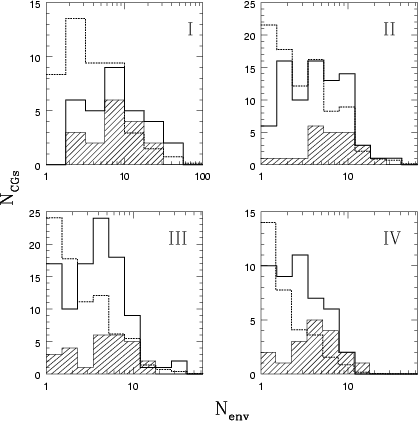
In Fig. 10 the overall distribution of CGs with respect
to
,
thereby reducing the number of Ts and Ms in subsample I from 34 to 31 and from 21 to 17 respectively.
In Fig. 10 the overall distribution of CGs with respect
to
![]() is shown.
The solid line refers to Ts, the hatched area to Ms.
It clearly emerges that Ts are more likely than Ms to be found
in isolated environments, but that, compared to the much more numerous
single galaxies (hatched line), their environment is denser.
According to the KS test differences between Ts and Ms
are significant at 98%, 97% and 94% c.l. in subsamples II,
III and IV, whilst they are non significant in class I.
In simulated samples Ms show no excess of neighbours
with respect to Ts, so that no corrections for selection effects
have to be applied to the environmental data.
Thus we find three independent parameters
(velocity dispersion, spectral properties and environmental
density) suggesting that Ts and Ms constitute different populations.
The sparser environment, the higher emission line fraction and the lower
velocity dispersion of Ts all might result from
high contamination by field interlopers.
However they are also compatible with Ts being recently formed systems
of field galaxies, not yet embedded within a common virialized halo,
in which dynamical friction efficiently
transfers orbital energy of the group into the internal energy of a
single merger remnant.
is shown.
The solid line refers to Ts, the hatched area to Ms.
It clearly emerges that Ts are more likely than Ms to be found
in isolated environments, but that, compared to the much more numerous
single galaxies (hatched line), their environment is denser.
According to the KS test differences between Ts and Ms
are significant at 98%, 97% and 94% c.l. in subsamples II,
III and IV, whilst they are non significant in class I.
In simulated samples Ms show no excess of neighbours
with respect to Ts, so that no corrections for selection effects
have to be applied to the environmental data.
Thus we find three independent parameters
(velocity dispersion, spectral properties and environmental
density) suggesting that Ts and Ms constitute different populations.
The sparser environment, the higher emission line fraction and the lower
velocity dispersion of Ts all might result from
high contamination by field interlopers.
However they are also compatible with Ts being recently formed systems
of field galaxies, not yet embedded within a common virialized halo,
in which dynamical friction efficiently
transfers orbital energy of the group into the internal energy of a
single merger remnant.
Copyright ESO 2002