Dipartimento di Astronomia, Università di Bologna, via Ranzani 1, 40127 Bologna, Italy

Abstract
Applying an automatic neighbour search algorithm to the 3D UZC galaxy catalogue (Falco et al. 1999) we have identified 291 compact groups (CGs) with radial velocity between 1000 and 10 000 km s $^{\rm -1}$ . The sample is analysed to investigate whether Triplets display kinematical and morphological characteristics similar to higher order CGs (Multiplets). It is found that Triplets constitute low velocity dispersion structures, have a gas-rich galaxy population and are typically retrieved in sparse environments. Conversely Multiplets show higher velocity dispersion, include few gas-rich members and are generally embedded structures. Evidence hence emerges indicating that Triplets and Multiplets, though sharing a common scale, correspond to different galaxy systems. Triplets are typically field structures whilst Multiplets are mainly subclumps (either temporarily projected or collapsing) within larger structures. Simulations show that selection effects can only partially account for differences, but significant contamination of Triplets by field galaxy interlopers could eventually induce the observed dependences on multiplicity.

Small galaxy systems such as pairs and Compact Groups (CGs) constitute the very lowest end of the clustering hierarchical scale. Given their high galaxy density and small velocity dispersion most CGs are expected to separate from their underlying background, become bound systems and ultimately collapse within a few crossing times. Actually the high frequency (or extreme longevity) of CGs can match the rather short lifetimes predicted by merger simulations (Barnes 1989) simply by varying the fraction of dark matter distributed through the group (Mamon 1987; Athanassoula et al. 1997; Zabludoff & Mulchaey 1998), assuming continuous accretion of infalling galaxies (Governato et al. 1996), or assuming that CGs are dense configurations that form temporarily within loose groups (Diaferio et al. 1994). An alternative scenario requires that merging CGs are continuously replaced by new forming ones (Mamon 2000).

To date it is difficult to further constrain the relative importance of parameters and correlations entering the modelling of CGs, essentially because no definite conclusions concerning fundamental properties of CGs have been achieved. A large unbiased sample is needed to provide statistically reliable answers to questions such as: Do isolated CGs really exist? And how does the request for minimum multiplicity depend upon magnitude and morphological classification of member galaxies? Hence, questions related to a proper choice of CG selection parameters become fundamental, whilst actually, these parameters are generally chosen according to criteria aiming at reducing contamination by non-physical structures. Indeed, the bound status of CGs is difficult to establish. CGs, unlike galaxy clusters, though presenting adequate mass density profiles, are generally too close (z<0.1) to induce efficient gravitational lensing phenomena (Mendes de Oliveira & Giraud 1994; Montoya et al. 1996), while concerning X-ray properties, diffuse emission tends to be associated only with embedded CGs in loose configurations that contain at least one early-type galaxy (Ponman et al. 1996; Mulchaey 2000; Heldson & Ponman 2000). Other tracers of a common potential well, such as HI or CO, are at present available only for a limited number of CGs (Williams & Rood 1987; Oosterloo & Iovino 1997; Verdes-Montenegro et al. 2001).

Therefore proximity in projected and redshift space, although affected by small number statistics, peculiar motions and interlopers (Moore et al. 1993; Diaferio et al. 1994), still remains the main tracer of physical association between galaxies in CGs. Interaction patterns and kinematical peculiarities between member galaxies constitute an a posteriori probe of physical association.

Because of the difficulty in identifying high redshift CGs, only low redshift CG samples are so far available. The best studied CG sample (HCGs, Hickson 1982, 1997) contains 92 CGs showing extremely heterogeneous characteristics. HCGs have been visually selected (according to multiplicity, isolation and luminosity concordance of member galaxies) and thus reflect some of the systematic biases intrinsic to identification of systems on the basis of their bidimensional distribution only. In order to overcome these biases automatic identification of CGs has been performed on a deep 2-D southern catalogue (SCGs, Prandoni et al. 1994; Iovino et al. 1999) and on 3-D catalogs (RSCGs, Barton et al. 1996, 1998). These studies intended to produce large CG samples by (partial) parametrical reproduction of Hickson's selection criteria. Hickson's isolation criterion has been slightly relaxed by Iovino et al. (1999) and not included at all by Barton et al. (1996), who additionally, included triplets among CGs. Triplets are structures generally excluded in bidimensional selected CG samples because, apart from the expected high contamination by superposed fore/background galaxies, they might represent a collection of unrelated field galaxies, rather than a physical structure (Diaferio et al. 1994). The Catalogue of Triple Galaxies (Karachentseva et al. 1979; Karachentseva & Karachentsev 2000) constitutes the exception, but because of poor number statistics affecting dynamical parameters, Triplets have so far been investigated mainly in relation to their high peculiar galaxy content. Recent availability of a 3-D large galaxy sample, including nearly 20 000 redshifts for northern galaxies brighter than m_B=15.5 (UZC, Falco et al. 1999), allowed us to construct a large CG sample selected on the basis of their compactness only. In selecting the sample we did not try to reproduce any of Hickson's criteria except compactness, in order to check if and at which level the properties of CGs are linked to multiplicity, to the large scale environment and to the luminosity and spectral properties of member galaxies.

The CG selection algorithm is described in Sect. 2. In Sect. 3 we describe the UZC catalogue and the prescriptions for the algorithm input parameters. The analysis of the characteristics of Triplets (Ts) and Multiplets (Ms) are presented in Sect. 4. In Sect. 5 statistical reliability of the CG sample is discussed. In Sect. 6 spectral properties of CG galaxy members are presented. CGs large scale environment and surface density contrast are analysed in Sects. 7 and 8 respectively. In Sect. 9 the relation between adopted selection parameters and the properties of the resulting CG sample are discussed. Conclusions are drawn in Sect. 10.

A Hubble constant of $H_{\rm0}=100~h^{\rm -1}$ km s $^{\rm -1}$ Mpc $^{\rm -1}$ is used throughout.

2 The CG identification algorithm

In order to safely deal with CG multiplicity and properly compare T and M characteristics we have devised a CG identification algorithm imposing compactness as the only requirement. The algorithm counts neighbours to each galaxy in 3D space within a volume defined by projected distance $\Delta r$ and velocity "distance'' $\Delta v^{\rm I} (\Delta r$ and $\Delta v^{\rm I}$ are free input parameters). When a galaxy is found to have at least two neighbours the geometrical center of the system is identified. Additional members within $\Delta r$ and $\Delta v^{\rm I}$ of the centroid are then searched for and a new center computed. This is an iterative process that goes on until convergence is reached, i.e. no further CG member is detected and no previously identified CG member gets excluded. Non-convergent systems are obviously rejected. CG centers are not weighted by magnitude of member galaxies on purpose, in order to enable non-biased investigation of possible relationships linking CG kinematics to luminosity.

The searching method is asymmetric and may produce different grouping depending on which galaxy is selected first. In order to overcome this undesirable effect the algorithm retains in the main sample only CGs whose single galaxies all have no further neighbour (within $\Delta r$ and $\Delta v^{\rm I}$ ) except those already listed as members. Non-symmetric CGs are excluded, because without definition of further selection criteria, the algorithm is unable to define which galaxies are CG members and which are to be left outside. The symmetrization procedure also ensures that no overlapping CGs are retained. Finally, cross correlation with ACO clusters (Struble & Rood 1999) enables the algorithm to exclude from the sample CGs which are cluster substructures at distance less than 1 $R_{\rm Abell}$ from the ACO centers.

For each CG the local surrounding galaxy density is computed within the free input parameters $\Delta R$ and $\Delta v^{\rm II}$ . The algorithm also provides parameters indicative of average compactness and maximum physical extensions. These are the unbiased line of sight velocity dispersion $\sigma _{v}$ , the maximum difference in redshift space between a CG member and the center $\Delta v_{\rm max}$ , the radius ${\it r}_{\rm ave}$ measuring projected average galaxy distance from the center, and the radius ${\it r}_{\rm max}$ defined as the projected separation between the center and the most distant CG member galaxy. Average projected dimension of CGs ( $r_{\rm ave}$ ) is preferred to the median value, because having imposed a maximum physical extension to CGs, each galaxy distance should be equally weighted.

Our algorithm displays some analogies and differences with the friends of friends (FoF) group searching algorithm by Huchra & Geller (1982) and with the hierarchical procedure applied by Tully (1987). Like Tully (1987) our CGs are defined by internal conditions only and our procedure starts hierarchically by requiring a minimum galaxy density threshold to identify a CG. At variance with the FoF method, requiring a maximum galaxy-galaxy separation as a function of redshift, we impose a maximum size for the CGs. Adopting a common scale for structures allows to safely deal with multiplicity but induces a redshift luminosity dependence. To correct for this bias the CG sample is divided in 4 distance classes (see Sect. 3) and the comparison of CGs of different multiplicity is performed within each class. Moreover while the FoF procedure, to discriminate between physical and non physical systems, requires a minimum density contrast threshold (computed with respect to the average galaxy density of the sample), our CGs are identified without a constraint on density contrast. Instead, we do compute the surface density contrast locally (within $\Delta R$ and $\Delta v^{\rm II}$ ) after CGs have been identified. The advantage of this approach is that we can perform non biased analysis of CG environments.

3 The CG sample

The CG sample we present here is specifically designed to allow comparison between compact Triplets and higher order CGs. Therefore, we have chosen to set $\Delta r=200~h^{\rm -1}$ kpc and $\Delta v^{\rm I}=\pm 1000$ km s $^{\rm -1}$ . The prescription for $\Delta$ r accounts for possible huge dark haloes tied to bright galaxies (Zaritsky et al. 1997; Bahcall et al. 1995). The value for $\Delta v^{\rm I}$ is large enough to allow a fair sampling of the CG velocity dispersion, which can be related to other observational parameters such as morphological content and surrounding galaxy density (Somerville et al. 1996; Marzke et al. 1995). Actually, more than 95% of the CGs display $\sigma _{v}$ values below 500 km s $^{\rm -1}$ .

Concerning the large scale, we have set $\Delta R=1~h^{-1}$ Mpc and $\Delta v^{\rm II}=\pm1000$ km s^-1 in order to map the environment on scales typical of loose groups/poor clusters. Moreover, adopting the same value for $\Delta v^{\rm I}$ and $\Delta v^{\rm II}$ ensures that each CG is sampled to the same depth of its large scale environment. Only CGs in a redshift range 1000 km s $^{\rm -1}$ to 10 000 km s $^{\rm -1}$ enter the sample. The low redshift threshold allows us to reduce uncertainties due to peculiar motions, the upper one to reduce the incidence of CGs with only extremely bright galaxies.

The search algorithm, applied to the UZC sample with the prescriptions just defined, yields a sample of 291 CGs: 222 Triplets (Ts) and 69 Multiplets (Ms) with more than 3 member galaxies. The algorithm additionally detected (and rejected) 56 ACO subclumps and 144 non-symmetric CGs, among which Ms are at least 50%. The CG sample is shown in Table 1 which lists RA and Dec of the center (Cols. 2 and 3), number of members n (multiplicity) (Col. 4), average projected dimension $r_{\rm ave}$ (Col. 5), mean radial velocity cz (Col. 6), unbiased radial velocity dispersion $\sigma _{v}$ (Col. 7) and, for CGs with $cz \geq 1500$ km s^-1 (see Sect. 7), the number of large scale neighbours $N_{\rm env}$ within $R=1~h^{\rm -1}$ Mpc (Col. 8). Cross identification with HCGs and RSCGs is reported in Col. 9. Table 2 lists member galaxies for each CG, their position, magnitude, radial velocity and spectral classification as reported in UZC. The CG sample characteristics are shown in Fig. 1.

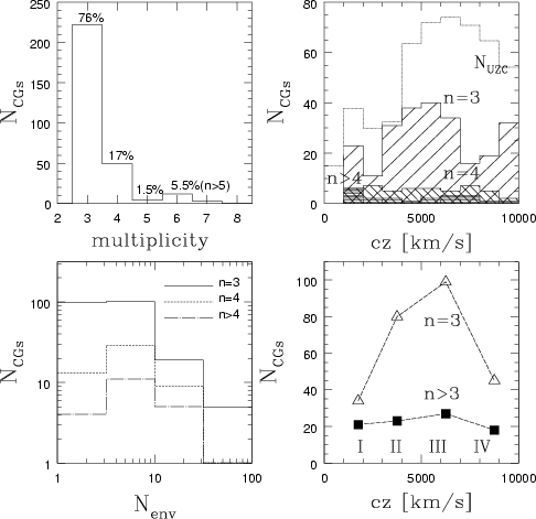$\begin{figure} \par\resizebox{\hsize}{!}{\includegraphics{focardifig1.ps}}\end{figure}$

Figure 1: In the upper left panel the CG distribution as a function of multiplicity is shown. The upper right panel shows redshift distribution for CGs with different multiplicity: Ts constitute 3/4 of the CG sample. The dotted line represents, on an arbitrary scale, the distribution of UZC galaxies. The lower left panel shows the number of large scale neighbours ( $N_{\rm env}$ ) for Ts, for CGs with 4 members, and for CGs with more than 4 members respectively. Ts constitute the majority of structures with few neighbours. In the lower right panel the number of Ts and Ms is plotted, within each of the 4 distance classes in which separate data comparison is performed.

Open with DEXTER

The CG distribution as a function of multiplicity (upper left panel) shows that Ts represent the majority of the sample. The upper right panel shows how the redshift distribution of CGs of different multiplicity compares to redshift distribution of UZC galaxies. The lower left panel shows the relation between CG multiplicity and the number of large scale neighbours $N_{\rm env}$ . A correlation between multiplicity and large scale environment clearly emerges, with Ts representing the majority of the structures with few neighbours. The KS test indicates that distributions between Ts and higher multiplicity CGs are different with significance level larger than 99.7%.

To extract physical information from the complete flux limited sample the role of the luminosity of member galaxies has to be properly disentangled, hence nearby CGs have to be separated from more distant ones. With this aim the sample was split into 4 distance classes whose radial velocities span over a 3000 km s^-1 range each, with an overlap among adjacent samples of 500 km s^-1. The first subsample is actually slightly smaller because all CGs at redshift below 1000 km s^-1 are excluded, and its overlap with the next subsample slightly larger. The 4 subsamples lie within 1000-3000 km s^-1, 2000-5000 km s^-1, 4500-7500 km s^-1, and 7000-10 000 km s^-1 respectively (henceforth referred as subsamples I, II, III and IV). Subsamples mimic homogeneous samples, complete in magnitude and volume, and allow to correctly take into account multiplicity and neighbour density. The small overlap in redshift space does not bias the statistical analysis of the sample, as only Ts and Ms within the same subsample are compared, and no comparison between CGs in different subsamples is performed. Table 3 reports for each subsample the median value of the kinematical parameters provided by the algorithm, together with the median value of the large scale neighbours. The distribution of Ts and Ms, in the four defined distance classes, is shown in the lower right panel in Fig. 1. The decline in both distributions in subsample IV reflects the sharply decreasing luminosity function of galaxies at the high luminosity end. The fraction of UZC galaxies in CGs within each of the 4 defined subsamples is 11%, 10%, 7% and 4% respectively. Actually, since the volumes covered are extremely different, our results on the 4 subsamples exhibit different levels of statistical significance. Subsample I should strongly reflect our position within the Local Supercluster. For example, several CGs in subsample I are Virgo cluster subclumps (see Mamon 1989).

The volume number density of all CGs (computed for systems at $cz\ge 2500$ km s^-1 and $\vert b_{\rm II}\vert\geq 40\hbox{$^\circ$ }$ ) turns out to be $1.6\times10^{\rm -4}~h^{\rm 3}$ Mpc^-3, almost 4 times the density of Ms alone. CGs number density slightly exceeds values estimated in RSCGs (Barton et al. 1996), which in turn, retrieve number densities much higher than in HCGs because of Hickson's bias against Ts.

Table 3: CGs kinematical and environmental parameters. The CG sample has been split according to redshift range. Figures for Ts and Ms are shown separately. Median values are tabulated.
subsample Ts $\sigma _{v}$ $\Delta v_{\rm max}$ $r_{\rm ave}$ $r_{\rm max}$ $N_{\rm env}$ Ms $\sigma$ _v $\Delta v_{\rm max}$ $r_{\rm ave}$ $r_{\rm max}$ $N_{\rm env}$

II 80 128 141 74 99 3 23 245 279 82 135 5

III 99 152 175 65 93 3 27 262 380 82 121 4

IV 45 174 200 79 109 2 18 314 446 91 122 3

**Table 3:** CGs kinematical and environmental parameters. The CG sample has been split according to redshift range. Figures for Ts and Ms are shown separately. Median values are tabulated.
subsample	Ts	$\sigma _{v}$	$\Delta v_{\rm max}$	$r_{\rm ave}$	$r_{\rm max}$	$N_{\rm env}$	Ms	$\sigma$ _v	$\Delta v_{\rm max}$	$r_{\rm ave}$	$r_{\rm max}$	$N_{\rm env}$
II	80	128	141	74	99	3	23	245	279	82	135	5
III	99	152	175	65	93	3	27	262	380	82	121	4
IV	45	174	200	79	109	2	18	314	446	91	122	3

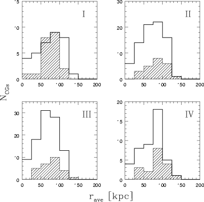$\begin{figure} \par\resizebox{\hsize}{!}{\includegraphics{focardifig2.ps}}\end{figure}$	Figure 2: Distribution of Ts and Ms (hatched) as a function of the parameter $r_{\rm ave}$ tracing the average projected dimension of the group.
Open with DEXTER

4 The main properties of CGs

$\begin{figure} \par\resizebox{\hsize}{!}{\includegraphics{focardifig3.ps}}\end{figure}$	Figure 3: Distribution of Ts and Ms (hatched) as a function of $\sigma _{v}$ , tracing the extension of the CG in redshift space.
Open with DEXTER

As far as kinematical properties are concerned, Fig. 2 shows the distribution of the average extension ( $r_{\rm ave}$ ) for Ts (solid histogram) and Ms (hatched) in the four subsamples. Ts appear more compact than Ms in all but the first subsample. However, according to the KS test, differences in $r_{\rm ave}$ between Ts and Ms are not significant (59%, 56% and 77% c.l. respectively). This is not unexpected, given our selection criteria, and actually confirms that we sample Ts and Ms on a common scale. When $r_{\rm max}$ rather than $r_{\rm ave}$ is examined differences get significant (above 90% c.l.) in subsamples II and III. While $\approx$ 40% of the Ms include a member which is at a distance larger than 150 h^-1 kpc from the center, this is the case for less than 7% of Ts. The excess of Ms with members close to the limiting distance, together with the high fraction of Ms among rejected non symmetric CGs, possibly indicates that we are sampling subclumps embedded in larger structures eventhough the external limit of 200 $h^{\rm -1}$ kpc imposed by the algorithm prevents from drawing definite conclusions concerning any typical dimensions for Ms. In the cz range between 2500 and 7500 km s^-1, including 60% of Ms, the average dimension of CGs increases with multiplicity following the relation $r_{\rm ave}\propto n^{\rm0.6}$ . This relation has been derived for the median number of galaxies in multiplets which is 4.5. The velocity dispersion of galaxies in a bound system provides an estimate of the potential well, although in CGs errors caused by random orientation of the system along the line of sight might dominate the result. In any case values obtained on a large sample of CGs are less affected by this bias, and thus yield more reliable results. In Fig. 3 the distributions of Ts and Ms relative to the parameter $\sigma _{v}$ are shown. Distributions are different at 61%, 99.6%, 97% and 98% c.l. respectively. Comparison of $\sigma_{\rm max}$ yields obviously more significant differences (98%, 99.99%, 99.9% and 99.8% c.l.). Considering again CGs within the range 2500-7500 km s^-1, we find $\sigma _{v}$ to increase with multiplicity as $n^{\rm 1.4}$ .

Next, before estimating the mass associated with CGs, we check whether and how many CGs in the sample satisfy the necessary (but not sufficient) criterion for a galaxy system to be virialized. In Fig. 4 $r_{\rm ave}/R_{\rm vir}$ as a function of $\sigma _{v}$ for Ts and Ms is plotted. $R_{\rm vir}$ is computed according to prescriptions in $\Lambda$ CDM ( $\Omega_{\rm M}=0.3$ , $\Omega_{\rm\Lambda}=0.7$ ) cosmologies, requiring a virialized system to display an overdensity greater than 333 with respect to the mean density of the universe. Figure 4 shows that most CGs (95%) in the sample satisfy the virialization condition and might therefore be physical bound systems. Had we compared $R_{\rm vir}$ with the harmonic radius, the fraction of virialized systems would be slightly lower (90%).

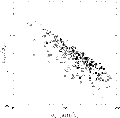$\begin{figure} \par\resizebox{\hsize}{!}{\includegraphics{focardifig4.ps}}\end{figure}$	Figure 4: Ratio of average dimension $r_{\rm ave}$ over virialization radius $R_{\rm vir}$ , as a function of the parameter $\sigma _{v}$ for Ts (empty triangles) and Ms (filled squares).
Open with DEXTER

Concerning the real nature of CGs it must also be stressed that the median velocity dispersion associated with galaxies in Ts (Table 3) is comparable to the mean galaxy-galaxy velocity difference associated with field galaxies (Somerville et al. 1996; Fisher et al. 1994). Accordingly one could speculate that the Ts sample suffers from serious contamination by pseudo-structures of unrelated field galaxies (filaments viewed nearly edge on), in which redshift tracing the Hubble flow is used to compute a velocity dispersion. If this is the case the contamination by interlopers is expected to bias the velocity dispersion of Ts towards the low end. However the exclusion of suspiciously low- $\sigma$ systems would also cause any genuine bound CG representing a system in its final state of coalescence to be excluded from the sample. In our sample the fraction of low $\sigma _{v}$ CGs (i.e. $\sigma_{ v}\leq 100$ km s^-1) turns out to be 32% and 16% among Ts and Ms. The first value is slightly lower than the 40% unbound Triplets claimed by Diaferio (2000). Figures are roughly consistent given that Diaferio selects systems with a FoF algorithm, which, when applied to small systems, tends to return an excess of elongated structures displaying enhanced contamination by outliers. Concerning Ms, the bias induced by interlopers might well push the velocity dispersion higher so that it is not obvious how to separate structures contaminated by interlopers from bound structures.

The substantial difference in the kinematical characteristics of Ts and Ms might affect also parameters directly derived from $\sigma _{v}$ and $r_{\rm ave}$ such as estimated mass ( $M \propto \sigma^2_{v}$ $\times r_{\rm ave}$ ) and dynamical time ( $H_{\rm0}t_{\rm d}\propto H_{\rm0}r_{\rm ave}/\sigma_{v}$ ). To compute these quantities we use $r_{\rm ave}$ instead of the harmonic radius $r_{\rm h}$ , because we select groups according to their maximal extension rather than constraining their maximum galaxy-galaxy separation. In Figs. 5 and 6 distributions of estimated M/L and $H_{\rm0}t_{\rm d}$ are shown. It appears that Ms possibly display higher M/L and shorter $H_{\rm0}t_{\rm d}$ than Ts, even though differences concerning these quantities are only marginally significant. The use of the harmonic radius (or of the median galaxy-galaxy separation) to compute these quantities would confirm the possible difference, with significance similar to that obtained with $r_{\rm ave}$ . The higher mean M/L associated with Ms could indicate either a higher mean $(M/L)_{\rm gal}$ or a higher fraction of mass between galaxies. Concerning $H_{\rm0}t_{\rm d}$ , the longer values associated with Ts might indicate that these are systems closer to turnaround, which are therefore less likely to be virialized. Alternatively the smaller M/L and higher $H_{\rm0}t_{\rm d}$ associated with Ts might well be claimed to arise because of contamination by interlopers, and hence to be non-physical.

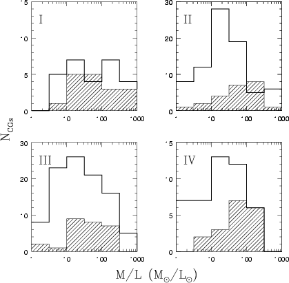$\begin{figure} \par\resizebox{\hsize}{!}{\includegraphics{focardifig5.ps}}\end{figure}$	Figure 5: M/L distribution of Ts and Ms (hatched). Ms display larger M/L than Ts at 46%, 98%, 87% and 94% c.l. in the four classes.
Open with DEXTER

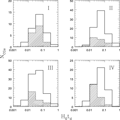$\begin{figure} \par\resizebox{\hsize}{!}{\includegraphics{focardifig6.ps}}\end{figure}$	Figure 6: Distribution of Ts and Ms (hatched) as a function of the dynamical time $H_{\rm0}t_{\rm d}$ in Hubble time units. Ms display shorter $H_{\rm0}t_{\rm d}$ than Ts at 42%, 86%, 90% and 98% c.l. in the four classes.
Open with DEXTER

In summary, the observed kinematical differences between Ts and Ms suggest that globally Ts do not constitute a fair subsample of Ms. Interestingly, differences are not significant between Ts and Ms in sample I, including mainly faint galaxies.

5 Simulated CG samples

$\begin{figure} \par\resizebox{\hsize}{!}{\includegraphics{focardifig7.ps}}\end{figure}$

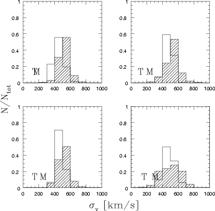Figure 7: Distribution of the median $\sigma _{v}$ in 300 pseudo CG samples (Ts, solid histogram and Ms hatched) identified in simulated UZC catalogues in which radial velocity have been randomly reassigned. The median value of the real T and M samples are indicated by the symbols T and M. The real sample, which is 3-4 times as large as the simulated ones, appear to include many more low $\sigma _{v}$ structures than reproducible by chance projection.

Open with DEXTER

In order to probe physical reliability of kinematical differences between Ts and Ms, pseudo-CG samples must be produced by running the search algorithm on a large set of randomized UZC catalogues. This allows us to correctly evaluate how much of the kinematical differences between Ts and Ms might be attributed to random properties of the UZC galaxy distribution. Yet, randomly generated catalogues (i.e. random assignment of RA, Dec and cz within the catalogue limits) would completely destroy large-scale structures in the nearby universe and hence would not constitute fair comparison samples. Random reassignment of UZC galaxy coordinates (including redshift) leads to more realistic representations.

In particular, to account for selection effects contaminating the velocity dispersion of T and M samples we have run the algorithm on 300 simulated UZC samples in which only the radial velocity of the galaxies has been reassigned. This leads to samples of $\approx$ 90 CGs ( $\rm median=95$ , 87 and 101 first and last quartile) and allows to reproduce separately structures on the (projected) sky and in redshift space. Median values of the velocity dispersion distribution in the 300 pseudo-CGs samples are displayed in Fig. 7, together with the median of samples of the real Ts (T) and Ms (M). It is evident that pseudo-CGs generally display $\sigma _{v}$ larger than observed in the real sample and that they are unable to reproduce the severe segregation observed between Ts and Ms. Accordingly, random properties do not account for the much lower $\sigma _{v}$ associated with Ts. Specifically, simulations indicate that for CGs between 2500 and 7500 km s^-1, $\sigma _{v}$ increases as $n^{\rm0.2}$ . Subtracting this contribution from the observed slope yields the true increase in $\sigma _{v}$ with multiplicity, which turns out to be $\sigma_{v}\propto n^{1.2}$ . Accounting for field interlopers, which should bias the velocity dispersion of Ts towards the low end, only slightly reduces the steep slope in $\sigma _{v}$ . Indeed, rejection of systems with $\sigma_{v}<100$ km s^-1 yields (after correcting for random contributions) $\sigma_{v}\propto n^{0.9}$ .

Simulations which keep the projected position of galaxies are unable to fairly account for random properties affecting the average dimension of CGs. Therefore additional simulations have been run, in which RA and Dec of UZC galaxies have been separately reassigned. In this kind of simulated catalogues an average of 15 CGs are retrieved. The increase of CGs average dimension with multiplicity turns out to be rather modest ( $\propto$ n^0.2). Subtraction of this contribution from the observed one gives the correct increase of $r_{\rm ave}$ with n ( $\propto$ n^0.4). The space-number density of CGs thus appears to slightly decrease ( $\rho\propto n^{-0.2}$ ) from Ts to Ms, a trend which is not consistent with the relation expected in constant space-number density structures. Conversely, a small increase in surface number density ( $\Sigma\propto n^{0.2}$ ) holds, which might be induced by our request for a common projected scale for CGs of different multiplicity.

6 Emission properties of galaxies in CGs

UZC labels homogeneously the spectral classification ( $E={\rm emission}$ lines, $A={\rm absorption}$ lines, B=E+A) for each galaxy, thereby allowing a check for possible links between emission properties and membership in CGs.

To test whether samples of Ts and Ms are intrinsically different, the fraction of emission (with or without absorption lines) to absorption galaxies can be compared. This fraction also represents a rough estimate of the incidence of young (or rejuvenated) over old objects, or alternatively of Spirals over Ellipticals. Figure 8 shows the Emission over Absorption (E/A) galaxy ratio for Ts (triangles) and Ms (squares) within each distance class. It is worth underlying that points in Fig. 8 indicate the ratio of the total population of emission galaxies over A galaxies in Ts and Ms.

It emerges that the fraction of emission over absorption galaxies decreases from sample I to IV. This trend towards a larger fraction of galaxies with emission spectra increasing for lower galaxy luminosities was already known to exist both in the optical (Zucca et al. 1997; Ratcliffe et al. 1998; Tresse et al. 1999) and in the near-IR (Mamon et al. 2001). Any comparison of the emission line galaxy fraction with respect to kinematical parameters has to account for this trend which, concerning morphology, was already reported by Tikhonov (1990), Mamon (1990) and by Whitmore (1992). However, Fig. 8 shows that, even when accounting for the decrease of emission line galaxies with redshift, Ts include higher fractions of emission line galaxies than Ms. The luminosity of Ts and Ms member galaxies being similar, the trend of increasing fraction of emission-line galaxies with decreasing multiplicity is probably real. Galaxies in Ts and Ms in sample I display no significant differences, in accordance with kinematical similarities between Ts and Ms in this subsamples.

Given that emission line galaxies are typically field galaxies, the data clearly suggest that Ts are more likely than Ms to be field structures (or to be contaminated by field interlopers) as already indicated by their lower $\sigma _{v}$ . To make this point more evident Fig. 8 additionally displays the E/A ratio for Single galaxies and for galaxies in CGs which are ACO subclumps (ACO $_{\rm CG}$ ). Single galaxies are UZC galaxies which turn out to have no UZC companion(s) within an area of 200 h^-1 kpc radius, and within $\Delta cz=\pm 1000$ km s^-1 and form a plausible comparison sample for CGs on small scales. Among UZC galaxies single galaxies are $\approx$ 10 times more numerous than CG galaxies. It clearly emerges that CGs, whatever their luminosity, are lacking in gas rich galaxies when compared to single galaxies, and that the deficiency is larger for Ms. At the same time Fig. 8 shows that CGs as a whole display an excess of spiral-rich galaxies when compared to those CGs which have been excluded from the sample because they turned out to be ACO $_{\rm CG}$ .

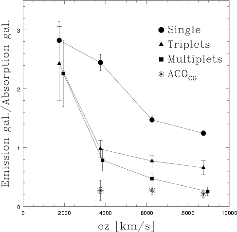$\begin{figure} \par\resizebox{\hsize}{!}{\includegraphics{focardifig8.ps}}\end{figure}$	Figure 8: Relative fraction of galaxies displaying Emission spectra over galaxies displaying Absorption spectra for Ts, Ms, for single galaxies in UZC (no neighbours within $r=200~h^{\rm -1}$ kpc) and for CGs that are ACO subclumps, which have been excluded from the main CG sample.
Open with DEXTER

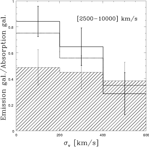$\begin{figure} \par\resizebox{\hsize}{!}{\includegraphics{focardifig9.ps}}\end{figure}$

Figure 9: Distribution of emission over absorption galaxy content as a function of CGs velocity dispersion. While in Ms (hatched area) the galaxy content is only modestly related to the velocity dispersion, the fraction of emission galaxies in Ts (solid histogram) turns out to be a strongly decreasing function of velocity dispersion. The hatched line shows the distribution for the whole CG sample.

Open with DEXTER

Our data show the existence of a trend from single galaxies to galaxies in cluster subclumps, in which CGs occupy an intermediate position. Figure 9, displaying the ratio of emission over absorption galaxies (in CGs at distance between 2500 and 10 000 km s^-1) as a function of CG $\sigma _{v}$ confirms that a morphology-velocity dispersion relation holds for the whole sample (hatched line), but also that the trend is induced by the inclusion among the CG sample of Ts (bold line) and specifically of low $\sigma _{v}$ Ts. Accordingly, any process linking the increase of $\sigma _{v}$ to the evolution of the spectral content of CGs is expected to be relevant predominantly in low multiplicity CGs. It is worth pointing out that if most low $\sigma _{v}$ Ts are non-real structures, the morphology-velocity dispersion relation is not retrieved. The morphology-velocity dispersion relation is similar to the morphology-density relation observed in clusters and loose groups (Dressler 1980; Postman & Geller 1984; Whitmore & Gilmore 1991) with the fraction of gas-rich galaxies being a strong signature of multiplicity. The morphology-density relation has previously been shown to hold for HCGs (Mamon 1986; Hickson et al. 1988) with an offset relative to the general Postman & Geller relation, indicating that at given spiral fraction, compact groups appear denser. It might be the inclusion within the sample of several spiral-rich, low multiplicity CGs that induces the offset, given that we find Ts to be even denser than Ms. Again, as for the morphology-velocity dispersion relation, the offset is to be reduced if most spiral rich, low $\sigma _{v}$ Ts are non-physical systems.

If the lower fraction of emission line galaxies in Ms corresponds to a lower fraction of Spirals, one accordingly expects the median $(M/L)_{\rm gal}$ of Ms members to be higher than for Ts galaxies. This could at least partially account for the higher M/L associated with Ms, although it remains uncertain whether the higher $\sigma _{v}$ and early type galaxy content associated with Ms do indeed indicate that these are systems more evolved than Ts. Multiplicity also appears to strongly influences the behaviour of systems in Hickson's sample. Specifically we have shown (Focardi & Kelm 2001) that the observed correlation between morphology and velocity dispersion in HCGs, (Hickson et al. 1988, 1992; Prandoni et al. 1994) just strongly reflects the different dynamical properties of systems with different multiplicity. In summary spectral characteristics indicate that two factors tend to strongly influence the number of emission line galaxies that will be retrieved in a CG sample. One is the fraction of faint galaxies included in the sample, with fainter galaxies being more likely to display emission line spectra. The second is the minimum multiplicity of CGs. The inclusion of Ts strongly biases a sample towards emission spectra galaxies. Combined with the average lower $\sigma _{v}$ , interactions between galaxies in Ts are accordingly predicted to be more disruptive than those in Ms, which suggests that perturbation patterns and/or asymmetric rotation curves (Rubin et al. 1991) should be more frequent among Ts.

7 Large scale environment of Compact Groups

Many embedded CGs are expected to be chance alignments of galaxies, not directly bound to one another along the line of sight, that form and destroy continuously within loose groups, whilst isolated CGs are generally assumed to be close dynamical systems, whose future evolution is a function of internal parameters only. Unfortunately, defining a CG as isolated is a non trivial problem, as one has to define boundaries (in space and luminosity) below which external galaxies perturb CG evolution and above which perturbations are negligible. Previous studies of CG environments yield contradictory results. Rubin et al. (1991) studying 21 HCGs find Ts to be more isolated than Ms. On the other hand Barton et al. (1996) do not confirm this result. However hardly any isolated CG should be retrieved, as bright galaxies are known to be strongly clustered, and faint galaxies are known to cluster around bright ones (Benoist et al. 1996; Cappi et al. 1998).

In order to properly investigate possible relations between small and large scale environments, the algorithm counts neighbours ( $N_{\rm env}$ ) for each CG within a distance $\Delta R=1~h^{-1}$ Mpc and $\Delta v^{\rm II}=\pm1000$ km s $^{\rm -1}$ from the CG center. To minimize distance uncertainties due to the relative incidence of peculiar motions neighbourhood richness is computed only for CGs at cz>1500 km s $^{\rm -1}$ , thereby reducing the number of Ts and Ms in subsample I from 34 to 31 and from 21 to 17 respectively. In Fig. 10 the overall distribution of CGs with respect to $N_{\rm env}$ is shown. The solid line refers to Ts, the hatched area to Ms. It clearly emerges that Ts are more likely than Ms to be found in isolated environments, but that, compared to the much more numerous single galaxies (hatched line), their environment is denser. According to the KS test differences between Ts and Ms are significant at 98%, 97% and 94% c.l. in subsamples II, III and IV, whilst they are non significant in class I. In simulated samples Ms show no excess of neighbours with respect to Ts, so that no corrections for selection effects have to be applied to the environmental data. Thus we find three independent parameters (velocity dispersion, spectral properties and environmental density) suggesting that Ts and Ms constitute different populations. The sparser environment, the higher emission line fraction and the lower velocity dispersion of Ts all might result from high contamination by field interlopers. However they are also compatible with Ts being recently formed systems of field galaxies, not yet embedded within a common virialized halo, in which dynamical friction efficiently transfers orbital energy of the group into the internal energy of a single merger remnant.

$\begin{figure} \par\resizebox{\hsize}{!}{\includegraphics{focardifig10.ps}}\end{figure}$	Figure 10: CGs distribution as a function of large scale neighbours. Neighbours have been counted out to R=1 h^-1 Mpc and $\Delta cz=\pm 1000$ from the CG center. The solid histogram refers to Ts, the hatched one to Ms. The dashed line shows the large scale environment distribution of single galaxies (on a scale that fits into the limits set by CGs).
Open with DEXTER

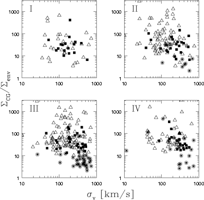$\begin{figure} \par\resizebox{\hsize}{!}{\includegraphics{focardifig11.ps}}\end{figure}$	Figure 11: Surface density contrast of Ts (empty triangles) and Ms (filled squares) versus velocity dispersion $\sigma _{v}$ . Stars represent ACO $_{\rm CGs}$ . The diagram clearly shows that CGs with different environmental and dynamical properties can be separated according to multiplicity.
Open with DEXTER

8 Surface density contrast

Next we combine information about multiplicity and environment and compute the surface density contrast of CGs ( $\Sigma_{\rm CG}/\Sigma_{\rm env}$ ), a parameter that quantifies the excess of surface density within the CGs as compared to that of their environment. It is defined as the surface number density of galaxies within and area of radius $r_{\rm max}$ with respect to the surface number density of galaxies within an area of radius 1 h^-1 Mpc. A space number density contrast constraint (defined with respect to the mean of the entire sample), has previously been coupled to the FoF algorithm to identify loose galaxy groups in the CFA (Ramella et al. 1989) and SRSS (Maia et al. 1989) surveys. If we were to adopt a similar criterion, CGs would correspond to even higher overdensities, because the vast majority of the systems defined on a 200 h^-1 kpc scale turn out to be single galaxies, which, as shown in Fig. 10, are associated with environments typically sparser than those of CGs. If surface density contrast is plotted against $\sigma _{v}$ one expects field systems to occupy low velocity dispersion-high density contrast regions and systems which are subclumps embedded within larger structures to occupy high velocity dispersion-low density contrast regions. In Fig. 11 the region occupied by CGs in a $\Sigma_{\rm CG}/\Sigma_{\rm env}$ vs. $\sigma _{v}$ plot is displayed. Whilst Ts are located predominantly near the field-systems area, Ms are typically associated with the embedded-systems area. Figure 11 shows that multiplicity is a rather robust parameter to discriminate between field structures and embedded structures, and indicates that, to reduce scatter in CG properties, Ts should not be included among higher multiplicity CGs, as this roughly would correspond to sampling together field-CGs and embedded-CGs.

In Fig. 11 the CGs that have been excluded from the sample because they are ACO subclumps are also plotted. ACO subclumps occupy a distinct region on the diagram. Whilst presenting a velocity dispersion similar to Ms, ACO $_{\rm CGs}$ are generally less overdense structures. On one side this might confirm that several Ms are structures that constitute the central core of large-groups/poor-clusters. This interpretation nicely matches observations indicating that, concerning X-ray properties, the distinction between compact and loose groups is not a fundamental one (Heldson & Ponman 2000). On the other hand the embedded status of many Ms could indicate that these are actually temporary chance alignments within a structure much larger than the CG (Mamon 1986; Walke & Mamon 1989; Hernquist et al. 1995). If this is the case, the characteristic $\sigma _{v}$ associated with Ms are probably too high an estimate, and all dynamically derived parameters, such as M/L or the dynamical time $H_{0}t_{\rm d}$ would strongly reflect the same bias.

To underline that the properties and differences between Ts and Ms are not to be attributed to random properties of the large scale distribution of UZC galaxies we show in Fig. 12 the position occupied by pseudo-CG samples extracted from simulated UZC catalogues (see Sect. 5) on a $\Sigma_{\rm CG}/\Sigma_{\rm env}$ vs. $\sigma _{v}$ plot. As pseudo-CG samples typically include few systems, to match the numerical dimension of the real sample we have grouped together 20 pseudo-CG samples.

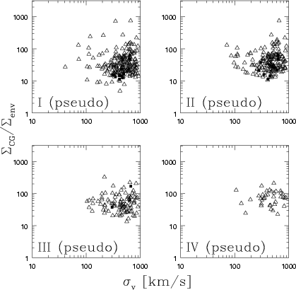$\begin{figure} \par\resizebox{\hsize}{!}{\includegraphics{focardifig12.ps}} \end{figure}$	Figure 12: Surface density contrast versus $\sigma _{v}$ in pseudo CG samples. To achieve numerical consistency with the real CG sample 20 pseudo-samples have been grouped together. No relation appears to exist between $\sigma _{v}$ and surface density contrast in CG samples identified in random UZC catalogs.
Open with DEXTER

9 Sample selection criteria and CGs properties

The different kinematical, morphological and environmental behaviour displayed by Ts and Ms allows us to relate commonly adopted CG selection criteria to the sample's properties.

Specifically our analysis has shown that multiplicity, velocity dispersion, large scale galaxy density and spectral/morphological mix are strongly linked together. Even if the explicit CG selection criterion constrains only one of these parameters, the link between them causes the remaining selection parameters to be constrained too. A constraint on compactness, such as the one we have adopted, biases a sample towards low multiplicity structures and thus indirectly towards low velocity dispersion, spiral rich, isolated structures. A small limit on the maximum velocity dispersion of CG members acts in the same direction. Therefore a parallel requirement for isolation though non affecting the low multiplicity CGs will severely reduce the number of high multiplicity CGs. Conversely, requiring a minimum of four members will bias a CG sample towards intrinsically embedded, spiral-poor groups.

Our analysis shows that Ms, whose parameters are statistically more reliable, happen to be more likely to constitute embedded subclumps whilst Ts might be more likely to be contaminated by systems which are just unbound projections of field galaxies. Interestingly, disregarding CGs in which faint members are counted (sample I), extremely compact systems with a minimum of 4 members which also fulfill the isolation criterion appear to be extremely rare indeed, thereby fitting predictions by numerical simulations claiming that compact configurations are rapidly destroyed (Mamon 1987; Barnes 1989).

Provided the fraction of non-physical CGs does not dominate the statistics, a large scatter in CG properties results when the analysis does not distinguish between Ts and Ms, as multiplicity appears to be a preliminary, robust discriminant between less evolved, field-systems and more evolved, embedded systems. Concerning HCGs, the suggestion that high and low $\sigma _{v}$ groups are intrinsically distinct can already be found in Mamon (2000), who further states that low $\sigma _{v}$ groups are either chance alignments or systems in their final stages of coalescence. The new point we add here is that low $\sigma _{v}$ systems are typically low multiplicity field structures.

That HCGs constitute a heterogeneous sample has previously also been stressed by de Carvalho et al. (1997) and Ribeiro et al. (1998), who, based on the analysis of 17 HCGs, identify 3 distinct CG families. They suggest that these correspond to 3 different dynamical stages, specifically they interpret embedded CGs as precursors of isolated and very dense systems. In comparison with Ribeiro et al. (1998) and based on our much larger CG sample we interpret low velocity dispersion, high overdense CGs (mostly Ts occurring along low density filaments) as the bottom level of the clustering process and embedded structures (either chance projections or collapsing cores within loose groups/poor clusters) such as systems in a more advanced evolutionary stage. Our interpretation, which explains the weak X-ray emission of field CGs in terms of their shallow potential wells (Heldson & Ponman 2000), requires that when X-ray emission is observed in small, gas rich CGs, it should be totally ascribable either to individual galaxies or to collisional shock-heating of the gas in low luminosity systems.

Our analysis indicates that interactions should be efficient mainly in the most overdense, low velocity dispersion structures, which are mainly Ts that include high fractions of gas-rich galaxies. Accordingly, it is not surprising that statistical analysis looking for interaction in HCGs (which include many n>3 CGs embedded within a common halo) globally reveals low fractions of merging remnants and blue Ellipticals (Zepf 1993). Actually, the suggestion that disturbances should be enhanced only among Ts better fits observations reporting that the most easily detected disturbed galaxies are spirals in small groups (Fried 1988) and that the most spectacular mergers, such as bright IRAS galaxies (ULIRGs), appear to involve strong interactions of gas-rich galaxies where the pairs are either isolated or part of small groups (Sanders & Mirabel 1996). It is also worth pointing out that the request for a minimum of 4 members which has biased the HCGs towards intrinsically embedded, gas-poor member groups, possibly explains why, despite the high expected interaction rate, HCGs as a whole present rather low evidence for strong AGN-starbursting episodes (Coziol et al. 1998; Kelm et al. 1998; Coziol et al. 2000).

Whether kinematical differences between Ts and Ms are generally compatible with hierarchical model predictions depends upon the specific assumptions one makes on the $(M/L)_{\rm gal}$ of Ts and Ms member galaxies and on the fractional group mass ( $f_{\rm gal}$ ) associated with its galaxies. Provided the luminosity of CG members is independent of multiplicity, and assuming $(M/L)_{\rm gal}$ and $f_{\rm gal}$ is the same for Ts and Ms, one predicts $r_{\rm ave}\propto N^{1/3}$ and $\sigma_{v}\propto N^{1/3}$ . While the $r_{\rm ave}$ slope is roughly consistent with these expectations, the $\sigma _{v}$ slope increases much faster. Indeed, Fig. 8 suggests that the assumption concerning the same $(M/L)_{\rm gal}$ for Ts and Ms is probably not satisfied, as absorption and emission galaxies are expected to represent ellipticals and spirals, and the former are typically associated with higher (M/L) galaxies than the latter. While $(M/L)_{\rm gal}$ is expected to increase with multiplicity, $f_{\rm gal}$ might actually decrease, due to the fact that higher multiplicity CGs are more likely to be associated with gas-rich, X-emitting groups. Consequently, before assessing whether globally data on CGs are (or are not) compatible with hierarchical model predictions, more accurate models, taking into account the different $(M/L)_{\rm gal}$ and $f_{\rm gal}$ of Ts and Ms, should be investigated.

10 Conclusions

We have taken advantage of a large, almost complete 3D catalogue to identify a sample of 291 northern CGs with redshift between 1000 and 10 000 km s $^{\rm -1}$ . CGs include a minimum of 3 members which have to lie within a region of 200 h^-1 kpc and $\Delta v=\pm 1000$ km s^-1. Kinematical properties of CGs and spectral characteristics of member galaxies have been investigated and related to large-scale environmental parameters. The sample has been used to compare Triplets, which constitute 76% of the sample, to higher-multiplicity structures. The analysis indicates that multiplicity is intrinsically linked to CG properties such as velocity dispersion, large-scale environment and spectral characteristics of galaxies. Specifically, it is found that Ts are more likely to be isolated systems and to display low velocity dispersion as well as a high gas-rich galaxy content. We suggest that Ts, although affected by interlopers, generally correspond to field galaxy structures. They constitute ideal sites for efficient merging to occur, and are thus likely to transform into a single galaxy as continuous accretion from surrounding galaxies is not viable on times shorter than their dynamical time scale.

On the other hand, higher multiplicity CGs are mainly associated with high velocity dispersion systems, whose members are preferentially gas-poor galaxies. These CGs display lower density contrast than field CGs and may thus suffer contamination by systems that are just temporary chance alignments within loose groups/poor clusters. Those Ms which are real physical systems should constitute the center of a larger collapsing group and are thus expected to display diffuse X-ray emission.

In summary, our data indicate that, provided most CGs are real physical systems, Ts and Ms correspond to two extremely different classes of systems. Therefore, any fair analysis of CGs properties should treat Ms and Ts separately.

Compact groups in the UZC galaxy sample

1 Introduction

2 The CG identification algorithm

3 The CG sample

4 The main properties of CGs

5 Simulated CG samples

6 Emission properties of galaxies in CGs

7 Large scale environment of Compact Groups

8 Surface density contrast

9 Sample selection criteria and CGs properties

10 Conclusions

References