A&A 390, 783-791 (2002)
DOI: 10.1051/0004-6361:20020754
B. Kerkeni![]()
Laboratoire "Atomes et Molécules en Astrophysique'', CNRS
UMR 8588 - DAMAp, Observatoire de Paris,
Section de Meudon, 92195
Meudon, France
Received 5 February 2002 / Accepted 13 May 2002
Abstract
Multipole relaxation and transfer rates due to isotropic collisions
with neutral hydrogen atoms are calculated and a general expression for
the hyperfine-structured levels are obtained.
Evaluation of these rates has been carried out using accurate
potential energy curves. The formulae given here for the depolarizing
collisional rates should be useful for accurately modelling the complex
linear polarization pattern of the Na I doublet in a complement to the
ground state's depolarizing collisional rates which were presented in a
previous paper (Kerkeni et al. 2000) hereafter referred to as Paper I.
Similarly the depolarizing collisional rates of the Mg I, Ca I, Sr I
resonance lines should be useful for polarization studies.
Key words: line: formation - polarization - atomic processes - Sun: atmosphere
Recent observations of scattering polarization on the Sun have revealed the existence of "enigmatic'' linear polarization signals in several spectral lines, which have motivated new theoretical investigations on atomic polarization and the Hanle effect (see e.g., the recent reviews by Trujillo Bueno 1999; 2001). Probably the most popular observational example is the case of the D1 and D2lines of Na I (see Stenflo & Keller 1997). Soon after the publication of such "enigmatic'' observations, Trujillo Bueno & Landi Degl'Innocenti (1997) showed, by means of selfconsistent radiative transfer calculations, that anisotropic radiation pumping processes in the solar atmosphere can lead to significant amounts of ground-level polarization, and to linear polarization signals in spectral lines with amplitudes in the observable range. In fact, Landi Degl'Innocenti (1998) could show, by adjusting of few free parameters, that a certain amount of ground-level atomic polarization in the hyperfine structure components of the ground level of sodium leads to a fairly good fit of the above-mentioned observations of linear polarization across the sodium doublet. More recently, Trujillo Bueno et al. (2002) have clarified the true physical origin of the ground-level polarization of Na I by carefully investigating, within the framework of the quantum theory of polarization, how it is actually produced, and modified by the action of a magnetic field of given strength and inclination.
Because isotropic collisions with the H atoms present in the stellar atmosphere contribute to depolarization of the atomic energy levels, a rigorous interpretation of the polarization spectra is possible only if the effects of the depolarizing collisions predominantly with H atoms are well understood for the spectral lines under consideration. In this paper we give the elastic and inelastic collisional rates of interest for the interpretation of the Na I, Mg I, Ca I, and Sr I resonance lines. Section 2 gives a brief introductory overview to familiarize the reader with the basic theoretical concepts and techniques applied for the computation of depolarizing rates caused by collisions with H atoms. Section 3 discusses the potential energy curves, while Sect. 4 focuses on the details of the applied theory. Finally, we show the results in Sect. 5, and summarize our main conclusions in Sect. 6.
Nowadays evaluating potential energy curves is the only obstacle to overcome to perform collisional calculations. Obtaining accurate values of these potential energy curves yield reliable relaxation parameters. The potential energy curves presented here have been calculated in the Born-Oppenheimer approximation (Born & Oppenheimer 1927) and obtained by methods of quantum chemistry (Schaeffer 1977; Jensen 1999). The electronic Schrödinger equation was solved by variational techniques for each internuclear distance giving the electronic energies as eigenvalues. The electronic wave function was obtained by using state average MultiConfiguration Self Consistent Field (MCSCF) method (Werner & Knowles 1985, 1988) which is a natural extension of the one-configuration Self Consistent Field (SCF) method.
At the SCF level, the electronic wave function is an antisymmetrical product of orbitals and electron spin functions and is given by a single determinant (Slater determinant) or configuration. Molecular orbitals that describe the wave function of each electron are determined by the field of the nuclei and the field arising from the average distribution of all the electrons. They are expanded in terms of atomic orbitals (LCAO method) built from a set of Gaussian functions (Boys 1950) in order to facilitate numerical integration. Optimization of the expansion coefficients for each internuclear distance is obtained by minimization of the energy of the electronic state. SCF wave functions give poor value for the relative energies, particularly for large internuclear distances.
To obtain a
better accuracy, one must go beyond the SCF level. This can be
done by using MCSCF wave functions given by a linear
combination of determinants (configurations) built on a set of
spinorbitals possibly larger than the set of orbitals occupied
in the SCF configuration. Molecular orbitals as well as
coefficients of the determinants are optimized at each
internuclear distance. This MCSCF approach takes into account a
large part of the correlation energy between electrons. In the case of very shallow potential energy curves (like ![]() states of NaH), the more accurate MultiReference Configuration Interaction method (MRCI) that includes all the single and double excitations from the MCSCF wave function is used. All the results were obtained using the MOLPRO
package
states of NaH), the more accurate MultiReference Configuration Interaction method (MRCI) that includes all the single and double excitations from the MCSCF wave function is used. All the results were obtained using the MOLPRO
package![]() .
.
![\begin{figure}
\par\includegraphics[width=8.8cm,clip]{aa2344f1.eps}
\end{figure}](/articles/aa/full/2002/29/aa2344/img17.gif) |
Figure 1: Potential energy curves for NaH. |
| Open with DEXTER | |
![\begin{figure}
\par\includegraphics[width=8.8cm,clip]{aa2344f2.eps}
\end{figure}](/articles/aa/full/2002/29/aa2344/img18.gif) |
Figure 2: Potential energy curves for MgH. |
| Open with DEXTER | |
![\begin{figure}
\par\includegraphics[width=8.8cm,clip]{aa2344f3.eps}
\end{figure}](/articles/aa/full/2002/29/aa2344/img19.gif) |
Figure 3: Potential energy curves for SrH. |
| Open with DEXTER | |
Depolarization studies of Mg I, Ca I and Sr I resonance lines involve the excited 1P state only, the ground state 1S being unaffected by depolarizing collisions (because calcium has nuclear spin I=0). However, this is not strictly true for Mg I and Sr I but it may be a sufficiently good approximation because their most abundant isotope have indeed I=0; i.e. 90% for Mg I and 93% for Sr I. Concerning the Na I D lines, collisional depolarization occurs both in the ground state (3s 2S1/2) and in the excited states (3p 2P1/2 and 3p 2P3/2). Results have been published for the ground state (see Paper I).
For CaH, accurate ab initio potential energy curves were available (Chambaud & Lévy 1989).
For MgH, the relevant potential energy curves are the third
![]() and second
and second ![]() states dissociating to the Mg(3s3p 1P
states dissociating to the Mg(3s3p 1P
![]() S) limit at large internuclear distances (taking into account the ground state
S) limit at large internuclear distances (taking into account the ground state
![]() and an intermediate asymptote involving the Mg I atom in a triplet state (3s3p3P). The Gaussian basis set for the H atom comprised the (8s, 4p, 3d) set of Widmark et al. (1990) contracted to [4s, 3p, 2d]. For magnesium, the basis comprised the (14s, 10p) functions of Sadlej & Urban (1991) and the (5d, 4f) functions of Widmark et al. (1991) contracted to [7s, 5p, 4d, 3f]. The total number of contracted Gaussian functions was 86. The potential energy curves were calculated from state average MCSCF wave functions in the
and an intermediate asymptote involving the Mg I atom in a triplet state (3s3p3P). The Gaussian basis set for the H atom comprised the (8s, 4p, 3d) set of Widmark et al. (1990) contracted to [4s, 3p, 2d]. For magnesium, the basis comprised the (14s, 10p) functions of Sadlej & Urban (1991) and the (5d, 4f) functions of Widmark et al. (1991) contracted to [7s, 5p, 4d, 3f]. The total number of contracted Gaussian functions was 86. The potential energy curves were calculated from state average MCSCF wave functions in the
![]() active space.
active space.
For SrH, the potential energy curves of interest are the
![]() and
and ![]() states dissociating to the Sr(5s5p 1P
states dissociating to the Sr(5s5p 1P
![]() S) asymptote. This requires calculating five
S) asymptote. This requires calculating five
![]() and four
and four ![]() states due to the first asymptotes involving the Sr I atom in 1S, 1D, 3P and 3D states. The Gaussian basis set for the H atom comprised the (7s, 4p, 3d, 2f) of
Kendall et al. (1992) contracted to [5s, 4p]. For the Sr I atom, the basis includes the (11s, 15p, 10d, 6f) of Sadlej & Urban (1991) contracted to [4s, 9p, 4d]. The potential energy curves were calculated from MCSCF wave functions in the
states due to the first asymptotes involving the Sr I atom in 1S, 1D, 3P and 3D states. The Gaussian basis set for the H atom comprised the (7s, 4p, 3d, 2f) of
Kendall et al. (1992) contracted to [5s, 4p]. For the Sr I atom, the basis includes the (11s, 15p, 10d, 6f) of Sadlej & Urban (1991) contracted to [4s, 9p, 4d]. The potential energy curves were calculated from MCSCF wave functions in the
![]() active space.
active space.
Adiabatic potential energy curves for NaH have been determined using MRCI wave functions. The basis sets and active space used in these calculations are described in Paper I. The calculations concern the
![]() and a
and a
![]() states dissociating to the Na(3s 2S
states dissociating to the Na(3s 2S
![]() S) asymptote and the A
S) asymptote and the A
![]() B
B![]() b
b![]() and c
and c
![]() states dissociating to the Na(3p 2P
states dissociating to the Na(3p 2P
![]() S) asymptote.
S) asymptote.
The results for the three systems are presented in Figs. 1, 2 and 3. The main characteristics of these potential energy curves is the presence of a large well in the
![]() states due to the ionic configuration M
states due to the ionic configuration M
![]() (M
(M
![]() ,Sr+,Na+).
,Sr+,Na+).
In order to test the basis set and the active space, the minima ![]() of the attractive X
of the attractive X
![]() A
A
![]() b
b![]() states were determined for the well studied NaH system (see Sachs et al. 1975; Pesl et al. 2000; Leininger et al. 2000). A fit of the first vibrational levels gives the harmonic frequency
states were determined for the well studied NaH system (see Sachs et al. 1975; Pesl et al. 2000; Leininger et al. 2000). A fit of the first vibrational levels gives the harmonic frequency
![]() .
The
vibrational levels were obtained from numerical integration of the
radial Schrödinger equation using the Numerov method.
The calculated values of these spectroscopic constants are given in
Table 1 for comparison with the experimental and theoretical results.
Our constants agree well with the experiments and improve some of the available theoretical results.
.
The
vibrational levels were obtained from numerical integration of the
radial Schrödinger equation using the Numerov method.
The calculated values of these spectroscopic constants are given in
Table 1 for comparison with the experimental and theoretical results.
Our constants agree well with the experiments and improve some of the available theoretical results.
| State | Reference |
|
|
||||
|
X
|
this work | 3.57 | 1166.7 | 4.909 | 0.149 | 1.89 | 0 |
| (Sachs et al. 1975) | 3.61 | - | - | 0.135 | 1.878 | 0 | |
| (Meyer & Rosmus 1975) | 3.57 | 1172.3 | 4.88 | 0.132 | 1.92 | 0 | |
| (Huber & Herzberg 1979) | 3.57 | 1171.4 | 4.902 | - | 2.12 | 0 | |
| (Olson & Liu 1980) | 3.558 | 1171.8 | 4.927 | - | 1.922 | 0 | |
| (Orth et al. 1980) | 3.566 | 1171.4 | 4.902 | 0.1386 | - | 0 | |
| (Pesl et al. 2000) | - | 1171.968 | 4.90327 | 0.137 | - | 0 | |
| A
|
this work | 6.05 | 313.01 | 1.7362 | -0.0679 | 1.21 | 22 310 |
| (Sachs et al. 1975) | 6.19 | - | - | - | 1.203 | 22 122 | |
| (Olson & Liu 1980) | 5.992 | 320 | 1.735 | - | 1.239 | 22 568 | |
| (Huber & Herzberg 1979) | 6.062 | - | - | - | 1.41 | 22 719 | |
| (Orth et al. 1980) | 6.0346 | 317.56 | 1.712 | -0.09152 | - | 22 713 | |
| (Pesl et al. 2000) | - | 319.96 | 1.70553 | -0.0971 | - | - | |
b |
this work | 4.46 | 419.88 | 3.0402 | 0.239 | 0.13 | 31 044 |
| (Sachs et al. 1975) | 4.46 | 419.39 | 3.533 | 0.853 | 0.109 | 30 938 | |
| (Olson & Liu 1980) | 4.497 | 430.3 | 3.09 | - | 0.133 | 31 479 | |
| (Huber & Herzberg 1979) | 4.195 | 419 | - | - | - | 30 940 |
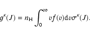
The potential energy curves described above were used to compute relaxation and transfer cross sections. Fully quantal close-coupling studies of the neutral systems Na-H, Mg-H, Ca-H ans Sr-H were performed using the formulation given by Mies (1973) and generalized by Launay & Roueff (1977).
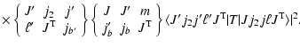
The radiating atom with angular momentum J collides with an H atom with angular momentum j2. We couple J and j2 to obtain the total angular momentum j of the two atoms. Owing to the invariance of the interaction potential V under rotations of the total system, the total angular momentum
![]() and its space fixed projection
and its space fixed projection ![]() are conserved during the collision. It is convenient to use scattering channel states
are conserved during the collision. It is convenient to use scattering channel states
![]() which describe the asymptotic fragments with relative angular momentum
which describe the asymptotic fragments with relative angular momentum
![]() .
The total wave function is expanded in terms of these channel states, the expansion coefficients are the radial amplitudes
.
The total wave function is expanded in terms of these channel states, the expansion coefficients are the radial amplitudes
![]() which satisfy the usual coupled
radial equations (Spielfiedel et al. 1991). This set of equations is always decoupled into two blocks as a result of parity conservation. In the calculations, we have assumed that the H atom remains in its ground 2S state
(L2=0,j2=1/2) and we have neglected collision-induced quenching to the other L states of the radiating atom. The scattering equations were solved subject to boundary conditions which define the T-matrix elements (Spielfiedel et al. 1991). The numerical method used is the Log Derivative Method (Johnson 1977).
Convergence was checked in terms of the range and step size in the scattering coordinate in the radial equations.
which satisfy the usual coupled
radial equations (Spielfiedel et al. 1991). This set of equations is always decoupled into two blocks as a result of parity conservation. In the calculations, we have assumed that the H atom remains in its ground 2S state
(L2=0,j2=1/2) and we have neglected collision-induced quenching to the other L states of the radiating atom. The scattering equations were solved subject to boundary conditions which define the T-matrix elements (Spielfiedel et al. 1991). The numerical method used is the Log Derivative Method (Johnson 1977).
Convergence was checked in terms of the range and step size in the scattering coordinate in the radial equations.
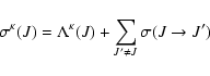
Under typical conditions of formation of strong resonance lines in stellar atmospheres, the interaction of the radiating atomic system with the perturbing gas is given by the relaxation matrix (Fano 1963). Under the assumption that the impact approximation is valid, the relaxation matrix ![]() is frequency independent and can be expressed in terms of collisional amplitudes (Nienhuis 1976) or collision T-matrix elements (Fano 1963). As the internal state distribution of the perturbers and the distribution of relative velocities are isotropic, the collisional relaxation of the atomic density matrix
is frequency independent and can be expressed in terms of collisional amplitudes (Nienhuis 1976) or collision T-matrix elements (Fano 1963). As the internal state distribution of the perturbers and the distribution of relative velocities are isotropic, the collisional relaxation of the atomic density matrix ![]() is fully isotropic. As a consequence, the relaxation matrix
is fully isotropic. As a consequence, the relaxation matrix ![]() is considerably simplified by using an expansion in components
is considerably simplified by using an expansion in components
![]() of irreductible tensorial sets (Fano 1949, 1954, 1957; Omont 1977; Blum 1981). We use here the same notations as in Paper I.
of irreductible tensorial sets (Fano 1949, 1954, 1957; Omont 1977; Blum 1981). We use here the same notations as in Paper I.
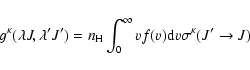
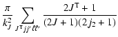
Due to the isotropy of the collisional relaxation, only the multipole components with the same value of ![]() and q are coupled, and the relaxation rate constants are q independent. Hence the relaxation equations may be written as:
and q are coupled, and the relaxation rate constants are q independent. Hence the relaxation equations may be written as:
 |
= | ||
| (1) |
For ![]() ,
,
![]() corresponds to collisional transfer of population
corresponds to collisional transfer of population
![]() ,
orientation
,
orientation
![]() and alignment
and alignment
![]() from state J' to state J.
from state J' to state J.
 |
(2) |
| = | |||
 |
(3) |
 | |||
 |
|||
 |
(4) | ||
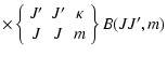
For J= J':
 |
(5) |
 |
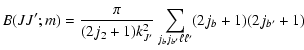
(6) |
![$\displaystyle \times \left \{\begin{array}{ccc}
m & J &J \\
\kappa &J &J \\
\end{array}\;\right\}]
B(JJ;m)$](/articles/aa/full/2002/29/aa2344/img75.gif) |
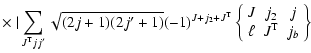
(7) |
| = |  |
||
| (8) |
Alkali earth atoms in a 1P state have an electronic angular momentum L=1 and an electronic spin S=0, so the angular momentum of the radiating atom is J=1. Combining J with the angular momentum j2=1/2 of the H atom, we obtain the total angular momentum j=1/2,3/2. The relevant channels for a total angular momentum ![]() are given in Appendix A. So, for each kinetic energy, two sets of three-channel scattering equations were solved for a given value of the total angular momentum
are given in Appendix A. So, for each kinetic energy, two sets of three-channel scattering equations were solved for a given value of the total angular momentum ![]() ranging from 1.5 to some suitable large value (up to 700.5 at the highest energies) in order to obtain convergence of the summation.
ranging from 1.5 to some suitable large value (up to 700.5 at the highest energies) in order to obtain convergence of the summation.
As inelastic cross sections to other states are negligible, we have only to consider the collisional relaxation rates of rank 0, 1 and 2. The corresponding cross sections are given by:
| (9) |
![\begin{figure}
\par\includegraphics[width=8.8cm,clip]{aa2344f4.eps}
\end{figure}](/articles/aa/full/2002/29/aa2344/img88.gif) |
Figure 4:
Relaxation rates
|
| Open with DEXTER | |
![\begin{figure}
\par\includegraphics[width=8.8cm,clip]{fig5.eps}
\end{figure}](/articles/aa/full/2002/29/aa2344/img89.gif) |
Figure 5:
Relaxation rates
|
| Open with DEXTER | |
![\begin{figure}
\par\includegraphics[width=8.8cm,clip]{fig6.eps}
\end{figure}](/articles/aa/full/2002/29/aa2344/img90.gif) |
Figure 6:
Relaxation rates
|
| Open with DEXTER | |
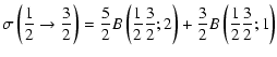
We give here the explicit expressions of the
![]() in terms of the Grawert coefficients B were given by Reid (1973) for J=1/2 and J=3/2.
in terms of the Grawert coefficients B were given by Reid (1973) for J=1/2 and J=3/2.
Explicit expressions of the tensorial tranfer cross sections between J=1/2 and J=3/2 states are the following:
 |
= | ![$\displaystyle \frac{1}{2\sqrt{2}}\left[3B\left(\frac{1}{2}\frac{3}{2};1\right)+5B\left(\frac{1}{2}\frac{3}{2};2\right)\right]$](/articles/aa/full/2002/29/aa2344/img96.gif) |
|
 |
= | ![$\displaystyle \sigma^1\left(\frac{1}{2}\rightarrow\frac{3}{2}\right)=\frac{\sqr...
...t(\frac{1}{2}\frac{3}{2};1\right)-B\left(\frac{1}{2}\frac{3}{2};2\right)\right]$](/articles/aa/full/2002/29/aa2344/img98.gif) |
|
 |
= | 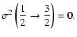 |
(10) |
 |
(11) |
The calculated relaxation rates, polarization transfer rates and fine structure transfer rate are presented in Figs. 7, 8 and 9. All these rates increase slowly with the temperature. As mentioned previously, the relaxation rates are larger than the transfer rates, the polarization transfer rate
g1(1/2,3/2) being almost negligible in comparison with the
![]() and
and
![]() coefficients. We remark that the differences between g1(1/2) and g3(3/2) are nowhere discernible to the resolution of the figure, this results from compensation of the two components of the relaxation cross sections (see Eq. (6)). The same trend was obtained by Wilson & Shimoni (1975) for Na(3p 2P
coefficients. We remark that the differences between g1(1/2) and g3(3/2) are nowhere discernible to the resolution of the figure, this results from compensation of the two components of the relaxation cross sections (see Eq. (6)). The same trend was obtained by Wilson & Shimoni (1975) for Na(3p 2P
![]() collisions. Table 2 shows a comparison of our calculated fine structure rate with previous results. We note a significant difference in these values due to the different potential energy curves used, nevertheless our values are very similar to those obtained by Monteiro et al. 1985 from potential energy curves that include correctly the ionic configuration in the
collisions. Table 2 shows a comparison of our calculated fine structure rate with previous results. We note a significant difference in these values due to the different potential energy curves used, nevertheless our values are very similar to those obtained by Monteiro et al. 1985 from potential energy curves that include correctly the ionic configuration in the
![]() molecular states. This indicates the importance of an accurate description of the potential energy curves in the intermediate and large internuclear distances.
molecular states. This indicates the importance of an accurate description of the potential energy curves in the intermediate and large internuclear distances.
| T(K) | 4000 | 4500 | 5000 | 6000 | 7000 | 8000 | 9000 | 10 000 |
| This work | 7.45 | 8.87 | 8.26 | 8.93 | 9.49 | 9.95 | 10.33 | 10.65 |
| (Monteiro et al. 1985) | - | - | 8.06 | 8.62 | 9.16 | 9.7 | 10.04 | - |
| (Roueff 1974) | - | 5.12 | - | 5.61 | 5.95 | - | 6.45 | 6.75 |
| (Lewis et al. 1971) | - | - | 3.03 | - | - | - | - | - |
The generalization of Eq. (2) with J=J' to include the effects of nuclear spin has
been studied by (Omont 1977). We consider the case of a single hyperfine
multiplet, with electronic angular momentum J and with nuclear spin I. The total angular momentum F takes the values
![]() and we may consider possible off diagonal
elements of the corresponding density matrix. The density matrix
and we may consider possible off diagonal
elements of the corresponding density matrix. The density matrix
![]() can be expanded as (Omont 1977):
can be expanded as (Omont 1977):
 |
(12) |
| TKQ(FF') | = | ||
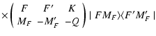 |
(13) |
The unitary transformation from the
basis
TKQ(FF') to the basis
![]() is given by:
is given by:
| TKQ(FF') | = | ||
 |
(14) |
| = | |||
 |
(15) |
![$\displaystyle {\frac{{\rm d} [\hfill^{(\lambda J)}\rho^{K}_{Q}(FF')]}{{\rm d}t} =-\sum _{
F''F'''}G_{K}(FF',F''F''')[\hfill^{(\lambda J)}\rho
^{K}_{Q}(F''F''')]}$](/articles/aa/full/2002/29/aa2344/img128.gif) | |||
| (16) | |||
| GK(FF', F''F''') = [(2F+1)(2F'+1)]1/2 | |||
 |
(17) | ||
| QK(FF',F''F''')=[ (2F+1)(2F'+1)]1/2 | |||
 |
(18) | ||
As previously mentioned in the case of the multipole relaxation of the hyperfine levels in the ground state the algebra coefficients are a fraction of one and thus all the collisional rates among the excited hyperfine levels are of the same order of magnitude as the
![]() coefficients of the fine structure 2P1/2 and 2P3/2 levels.
coefficients of the fine structure 2P1/2 and 2P3/2 levels.
![\begin{figure}
\par\includegraphics[width=8.5cm,clip]{fig7.eps}\par
\par\end{figure}](/articles/aa/full/2002/29/aa2344/img136.gif) |
Figure 7:
Relaxation rates
|
| Open with DEXTER | |
![\begin{figure}
\par\includegraphics[width=8cm,clip]{fig8.eps}
\end{figure}](/articles/aa/full/2002/29/aa2344/img137.gif) |
Figure 8:
Polarization transfer rate
|
| Open with DEXTER | |
![\begin{figure}
\par\includegraphics[width=8cm,clip]{fig9.eps}
\end{figure}](/articles/aa/full/2002/29/aa2344/img138.gif) |
Figure 9: fine structure rate versus temperature T(K). |
| Open with DEXTER | |
Cross sections were averaged over a Maxwell distribution of
velocities. The variation of the relaxation rates with
the temperature is very smooth and was found to increase as ![]() and is given as follows for 200 K
and is given as follows for 200 K ![]()
![]() K.
K.
Mg(1P![]() :
:
g1=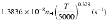 |
|
g2=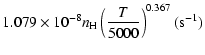 |
(19) |
Ca(1P)+H:
g1= |
|
g2=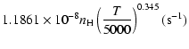 |
(20) |
g1=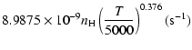 |
|
g2=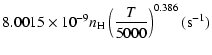 |
(21) |
| J=1/2 | 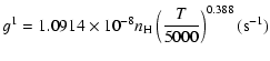 |
(22) | |
| J=3/2 | 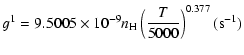 |
||
 |
|||
 |
(23) |
| = | |||
| = |  |
||
| = | |||
| = |  |
||
| = | |||
| = |  |
(24) |
As previously mentioned (see Paper I), depolarization in the ground level occurs for much lower densities (1014 cm-3). Of course, the correct diagnostic requires the resolution of the rate equations including radiative and collisional processes between hyperfine levels. This work is in progress (Kerkeni & Bommier 2002).
Acknowledgements
The advice and assistance of N. Feautrier and A. Spielfiedel is gratefully acknowledged. I wish to thank E. Landi Degl'Innocenti for helpful discussions. I acknowledge the referees for helpful comments that improved and clarified the understanding of the paper. The computations were performed on the work stations of the computer center of Observatoire de Paris.
| Parity |
|
|
||||
| J | j | channel | J | j | ||
| number | ||||||
| 1 |
|
|
1 | 1 |
|
|
| 1 |
|
|
2 | 1 |
|
|
| 1 |
|
|
3 | 1 |
|
|
| Parity |
|
|
||||
| J | j | channel | J | j | ||
| number | ||||||
|
|
1 |
|
1 |
|
0 | |
|
|
1 |
|
2 |
|
1 | |
|
|
1 |
|
3 |
|
1 | |
|
|
1 |
|
4 |
|
2 |
|
|
|
2 |
|
5 |
|
2 | |
|
|
2 |
|
6 |
|
2 |
|
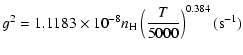
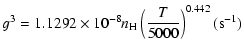
The variation of the hyperfine depolarizing rates with
the temperature is very smooth and was found to increase as ![]() and is given as follows for 200 K
and is given as follows for 200 K ![]()
![]() K.
K.
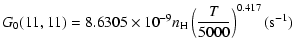
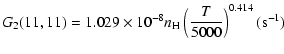
| J=1/2 |  |
||
 |
|||
 |
|||
 |
|||
 |
(C.1) |
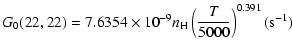
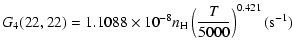
| J=3/2 |  |
||
 |
|||
 |
|||
 |
|||
 |
|||
 |
|||
 |
|||
 |
|||
 |
(C.2) |
 |
|||
 |
|||
 |
|||
 |
|||
 |
(C.3) |