A&A 389, 1039-1046 (2002)
DOI: 10.1051/0004-6361:20020595

Large-scale disturbance of the solar wind by a comet

R. Wegmann

Max-Planck-Institut für Astrophysik, 85748 Garching, Germany

Received 13 February 2002 / Accepted 26 March 2002

Abstract
Model calculations for the interaction of the solar wind with a comet are presented that extend 30 million km into the tail. It is shown that the disturbance of the interplanetary magnetic field (IMF) (the draping) is limited to timescales of 10 to 50 hours and length scales of 10 to 50 million km. This is supported by a theoretical argument about the acceleration of the cometary ions. The distribution of ions and protons at the end of the model tails agrees with measurements made by Ulysses far in the tail of comet Hyakutake. It is shown that the ion tail is concentrated in the current sheet between two flux lobes as long as the draping persists. The far tail, however, is flat and concentrated in a plane parallel to the IMF.

Key words: comets: general - Sun: solar wind

   
1 Introduction

The spacecraft Ulysses detected cometary ions on May 1, 1996, that most probably came from comet Hyakutake whose nucleus was 3.5 AU away (Gloeckler et al. 2000). At the same place a "density hole'' in the solar wind was found, with a drop of proton density of almost an order of magnitude and a comparable rise in proton temperature (Riley et al. 1998). An unusual magnetic field structure was detected simultaneously by the spacecraft's magnetometer (Jones et al. 2000). It was interpreted as the draped magnetic field of comet Hyakutake. On July 28, 2000, an interplanetary field enhancement was found by Ulysses at a heliocentric distance of 3.08 AU. It was tentatively attributed to a comet with small heliocentric distance which apparently escaped the attention of comet hunters (Jones et al. 2001).

Up to now there are no model calculations which extend so far into the tail, that they can describe the situation of the Ulysses encounter with comet Hyakutake's tail. In this paper we try to fill in this gap to some extent. We describe the tail up to a distance of about 0.2 AU from the nucleus. It turns out that the behaviour of the tail at such large distances cannot simply be inferred from previous model calculations, which covered only regions of about one million km size. Previous spacecraft encounters with comets are also not representative, since they sampled only a very narrow region in front of and behind the nucleus.

We concentrate in particular on the behaviour of the magnetic field. The comet drapes the interplanetary magnetic field (IMF) around the nucleus as predicted by Alfvén (1957). The draped field shapes the tail on scales of several million km to a flat ribbon squeezed between two flux ropes of opposite polarity (see e.g. Schmidt & Wegmann 1980; Fedder et al. 1983). The draped field transfers momentum via curvature forces from the bystreaming solar wind to the slow cometary ions. These are accelerated. As they catch up with the solar wind the draping decreases and vanishes. We show that this occurs on scales of several ten million km.

The plan of the paper is as follows: After a description of the numerical models in Sect. 2 we study the decay of the draping with model calculations in Sect. 3. In Sect. 4 we study theoretically the acceleration of cometary ions by the curvature forces of the magnetic field. The effect depends on solar wind conditions and cometary production rates. The deformation of the tail under the influence of the magnetic field is studied in Sect. 5. The ion composition in the far tail is considered in Sect. 6 and compared with the ion ratios observed by Ulysses. In the concluding Sect. 7 we summarize the results of the paper.

 

 

Table 1: Comet and solar wind parameters used in the models.

model		H1	H2	H3	H4
Comet:
gas production rate Q(H2O)	[1029 s-1]	20	10	5	2
helioc. dist. $r_{\rm h}$	[AU]	.35	.7	1	1.4
Solar wind:
density $n_{\rm sw}$	[cm-3]	17	12	10	5
electron temp. $T_{\rm e}$	[105 K]	2	2	2	1.5
proton temp. $T_{\rm p}$	[105 K]	1	1	1	.75
velocity $u_{\rm sw}$	[km s-1]	750	600	400	300
magnetic field $B_{\rm sw}$	[nT]	68	30	10	7
derived quantities:
Alfvén speed a	[km s-1]	360	189	69	68
sound speed c	[km s-1]	64	64	64	55
magnetosonic speed	[km s-1]	365	200	94	88
Mach number		2.05	3	4.3	3.4
eff. ionis. rate $\sigma_{\rm eff}$	[10-6 s-1]	3.05	2.00	1.39	0.50
interaction lengthscale $R_{\rm I}$ (1)	[105 km]	7.9	4.6	2.9	1.1
shock distance $R_{\rm S}$	[105 km]	5.9	6.5	5.5	3.8
estim. shock distance (Ma = 1)	[105 km]	4.3	3.4	2.6	1.8
acceleration time scale $t_{\rm a}$ (8)	[h]	8.0	13.5	42.1	12.4
acceleration length scale $l_{\rm a}$	[106 km]	21.6	29.1	60.6	13.4

   
2 Models

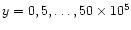
The models are calculated with the numerical method described by Wegmann (1995) on a rectangular non-uniform grid which is concentrated near the nucleus. All models are calculated on a $25 \times 25 \times 75$grid which extends $5.85\times 10^6$ km to the sides, $2.52\times 10^6$ km to the subsolar side and $30.86\times 10^6$ km into the tail. The resolution near the nucleus is 15 000 km. The magnetic cavity is not resolved.

We use a system of coordinates xyz centered on the nucleus with x along the Sun - comet axis, positive into the tail, with y parallel to the (transversal) IMF and z perpendicular to the xy-plane. We call the xy-plane the IMF plane and the xz-plane the perpendicular plane.

The cometary plasma flow is described by the MHD equations with source terms. A simple chemistry for the water group and for CO is implemented in a similar way as described by Wegmann et al. (1999). Ionisation by solar UV photons, by charge exchange with solar wind protons and by impact with solar wind electrons, is included.

Along the inflow boundary we prescribe solar wind conditions. On all other boundaries (on the sides and in the far tail) we use open boundary conditions, i.e., we assume that the values on the boundary are equal to the (calculated) values in the adjacent grid cell.

We calculate only models with transversal fields, and we neglect the motion of the comet. This is done for simplicity, since under these conditions the calculation can be restricted to a quadrant. But this simplification also helps to better isolate and demonstrate the effects. We are well aware that for comets at small heliocentric distances, the inclination of the field and the proper motion of the nucleus are important.

Table 1 shows the parameters of the calculated models. The model H1 is representative for comet Hyakutake near perihelion (Jones et al. 2000). The model H3 resembles comet Halley near the Giotto encounter. Model H4 is a small comet at larger heliocentric distance in a slow solar wind. The different solar wind conditions and heliocentric distances lead to different effective ionisation rates $\sigma_{\rm eff}$ which must be considered in estimates for the exhaustion of the neutral gas coma. The interaction scale length

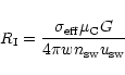$$% R_{{\rm I}}={\sigma_{\rm eff} \mu_{\rm C}G \over 4\pi w n_{\rm sw}u_{\rm sw}}$$ (1)

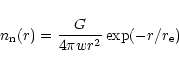
is a combination of the total production rate G, the mean molecular weight $\mu_{\rm C}$ of a cometary particle, the outflow velocity wof the neutrals and the density $n_{\rm sw}$ and velocity $u_{\rm sw}$ of the solar wind. It determines the shock distance $R_{\rm S}$. The shock distance can be estimated by the method of Schmidt et al. (1993) which also takes the influence of the IMF into account. The source Q(CO) of CO molecules is always assumed to be 10% of the water production rate Q(H₂O). Therefore, $G=1.1 \times$ Q(H₂O) and $\mu_{\rm C} =18.9$ in formula (1).

   
3 Draping of the magnetic field

The solar wind flow is decelerated by the pick-up of slow and heavy cometary ions. The mixture of solar wind protons, cometary ions and electrons is compressed in the stagnation region in front of the nucleus. The frozen-in fieldlines are hung up in the magnetic pile-up region and draped around the nucleus. The nucleus is a small massive obstacle of only about 10 km size. Outside the nucleus only the inertia forces of the pick-up ions brake the solar wind. This volatile ion cloud is connected via the magnetic fieldlines to the bystreaming solar wind flow and accelerated by curvature forces. As the flow is accelerated to solar wind velocity the draping of the field decreases and finally vanishes. Model calculations give information about the length scales and time scales of this process.

Figure 1 shows the field- and streamlines in a plane parallel to the IMF for the model H1 at a distance of 15 000 km from the IMF plane. There is strong draping at and behind the nucleus. But this draping vanishes as the field expands into the tail. The field strength and the velocity return to solar wind values at the end of the computational grid at a distance of 30 million km (=0.2 AU).

The stagnant field in the magnetic pile-up region brakes the flow. A region of high total pressure builds up in front of the nucleus. The pressure expands and accelerates the plasma in the y and z direction, so that it can flow around the nucleus. The velocity component along the field persists. This causes a strong lateral expansion of the flow (see streamlines in the right panel of Fig. 1). The flow across the field is braked by magnetic forces (see also Sect. 5) so that in the perpendicular plane the streamlines are almost straight with a deflection only around and close to the nucleus (see Fig. 2).

Figure 3 shows the same as Fig. 1 but for the model H4 of a small comet exposed to slow solar wind with low magnetic field. The draping of the field decreases but does not yet completely vanish at the end of the computed tail. The deflection of the streamlines is much less pronounced than in Fig. 1.

At larger distances from the IMF plane there are fewer pick-up ions. The solar wind flow is braked by the bow shock but then there is nothing to hang up the fieldlines. The fieldlines behave like strings which are excited and oscillate and radiate into the ambient solar wind. This is clearly visible in the fieldline pattern of model H1 at a distance of 1 million km from the IMF plane (see Fig. 4). To make this clearer we have drawn the deflection of several points along the fieldline as a function of time (Fig. 5). The maximum deflection is $3.7 \times 10^5$ km towards the sun. The deflection decreases. It goes to zero after about 4 hours. Then it overshoots and attains values of $1.3\times 10^5$ km in the tailward direction. The point on the plane of symmetry (y=0) attains its maximal deflection first, since it is first hit by the bowshock. The other maxima occur later. There is apparently a wave running outward along the fieldline. The central point turns back first, braked by curvature forces. The braking of the opposite motion comes from the ambient solar wind. The central point is the last to turn back from the tailward deflection. In the far tail the fieldline seems to approach asymptotically the rest state of a straight line again.

   
4 Acceleration of cometary ions

The kinetic energy of the solar wind is transformed in the bow shock to thermal energy. This pressure is sufficient to reaccelerate the solar wind to solar wind velocity. The cometary ions, however, need an additional force for acceleration. This is provided by the magnetic field which, due to the draping, transports momentum from the bystreaming solar wind towards the cometary tail.

We consider the x-component of the stationary momentum equation (recall that x is in the direction of the tail)

 

$$% \rho u_x {\partial u_x \over \partial x}= - \rho (u_y {\partial... ...artial p_{\rm mag} \over \partial x} +{1 \over \mu}({\vec B},{\rm grad}\;) B_x.$$ (2)

The term on the left side describes the change of u_x along the x-line, i.e., the acceleration. The first term (1) on the right side describes the effect of a change from one streamline to another, the second one (2) the braking by the addition of mass, the third (3) and fourth (4) the forces from gas and magnetic pressure gradients. The last term (5) is (basically) the curvature force of the magnetic field.

Figure 6 shows the different terms in Eq. (2). In the tail the acceleration is almost exclusively done by the curvature force (5).

On the sides, where the fieldlines are concave towards the solar wind, the solar wind exerts the force which is transferred by the field to the tail. If constant field strength $B=B_{\rm sw}$ is assumed, the force density is equal to $\kappa B_{\rm sw}^2/\mu$ with the curvature $\kappa$of the fieldline. The total force F(z) exerted onto a sheet parallel to the IMF plane at a distance z is

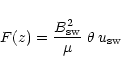$$% F(z) = {B_{\rm sw}^2 \over \mu}\; \theta\; u_{\rm sw}$$ (3)

where the "draping angle'' $\theta$ is the maximal angle by which the fieldline is deflected, i.e.,

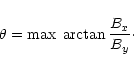$$% \theta =\max \;\arctan{B_x \over B_y}\cdot$$ (4)

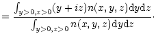
This force is available to accelerate the mass M(z) of pick-up ions added to the flow in this sheet. If we assume constant acceleration a(z) in the sheet, then it follows from F(z)= M(z) a(z) that the time t(z) needed to accelerate the ions to solar wind velocity $u_{\rm sw}$, is proportional to the added mass

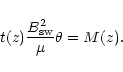$$% t(z) {B_{\rm sw}^2 \over \mu} \theta =M(z).$$ (5)

The factor of proportionality is up to a factor of order unity the inverse of the energy density $B_{\rm sw}^2/\mu$ of the IMF.

	Figure 1: Left: magnetic field strength [nT] and fieldlines in the model H1 at a distance of z= 15 000 km from the IMF plane. Right: velocity [km s-1] and streamlines. The length scale is in 105 km
Open with DEXTER

	Figure 2: Right: velocity [km s-1] and streamlines in the model H1 in the perpendicular plane. The red contour is for $u=u_{\rm sw}$. Left: the deflection (upper panel) and the velocity (lower panel) along the streamlines.
Open with DEXTER

	Figure 3: The same as Fig. 1 but for model H4.
Open with DEXTER

	Figure 4: The same as Fig. 1 but in a plane at a distance $.97\times 10^6$ km from the IMF plane.
Open with DEXTER

	Figure 5: The deflection of the fieldlines at $z=.97\times 10^6$ km (the same as in Fig. 4) at positions $y=0,5,\dots ,50\times 10^5$ km as a function of time. Maxima and minima are indicated by asterisks.
Open with DEXTER

	Figure 6: Upper panel: the velocity component ux [km s-1]. Lower panel: the different terms (force densities [10-18 dyn cm-3]) of Eq. (2) as functions of x along a line parallel to the axis at $y= z=.53\times 10^5$ km distance. The solid line is the left side of Eq. (2).
Open with DEXTER

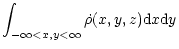
We derive now an approximation for the right hand side in (5). The density $n_{\rm n}$ of neutral particles at the distance r from the nucleus is given by

$$% n_{\rm n}(r)= {G \over 4 \pi w r^2} \exp(-r/r_{\rm e})$$ (6)

where $r_{\rm e}= w/\sigma_{\rm eff}$ is the length scale for the exhaustion of the neutral particles by ionisation. The source term $\dot \rho$ in the continuity equation is given by $\dot \rho= \sigma_{\rm eff}\; m_{\rm C}\; n_{\rm n}$with the mass $m_{\rm C} =\mu_{\rm C} \; m_{\rm p}$ of a cometary particle ($m_{\rm p}$ = proton mass). The mass added in the plane parallel to the IMF plane at a distance z is then

 

$$\int_{-\infty <x,y<\infty} \dot \rho (x,y,z) {\rm d}x {\rm d}y$$ M(z) =

$${\sigma_{\rm eff}\; m_{\rm C}\; G \over 2 w} E_1(z/r_{\rm e})$$ = (7)

with the exponential integral E₁ (see e.g. Abramowitz & Stegun 1984, formula 5.1.1 and Fig. 5.1).

Figure 7 shows for model H4 the mass source term calculated in the model and the approximation (7). The approximation is valid with a relative error of less than 1.58. For small distances the amount of added ions is limited by recombination processes. Therefore, the r^-2 singularity in $\dot \rho$and the $-\log z$ singularity in $E_1(z/r_{\rm e})$ do not occur. M(z) remains bounded as $z \to 0$. We can assume that $E_1(z/r_{\rm e}) \le 1$ over the range of interest and derive from (7) and (5) a time scale

$$% t_{\rm a}={\sigma_{\rm eff}\; m_{\rm C}\; G \over 2 w} {\mu \over B_{\rm sw}^2}$$ (8)

for the acceleration of the cometary tail to solar wind velocity. This occurs on the length scale $l_{\rm a}= t_{\rm a} u_{\rm sw}$. We have calculated these scales for our models and inserted the values into Table 1. The values are of the order 10 to 40 hours and 10 to 50 million km.

Since the solar wind can be reaccelerated by pressure forces alone, we can assume that the time when the tail reaches solar wind velocity roughly coincides with the time when the cometary ions are accelerated to this velocity. One can already see in Fig. 1 that even in the IMF plane the solar wind velocity is reached near the end of the computed tail. This occurs earlier in sheets further from the IMF plane. We have determined in the models for different values of z the time t₁ when the flow at the central line y=0 (starting at the upstream boundary of the grid at $2.5\times 10^6$ km distance) again reaches solar wind velocity. In Fig. 8 we have plotted this time against the added mass M(z). The relation is close to linear t₁=a₀+a₁M.

The flow is accelerated to velocities larger than $u_{\rm sw}$. The cometary plasma overtakes the solar wind, the fieldlines become convex towards the solar wind, which now acts as a brake (see Fig. 5) and tries to adjust the plasma velocity again. The mechanism for deceleration is the same as described before for acceleration. Therefore, the force is as in (3). One finds in the models that there is a similar linear relation t₂=b₀+b₁M for the time t₂ when the flow reaches solar wind velocity for the second time.

	Figure 7: The added mass M(z) in the plane parallel to the IMF plane at a distance z in the model H4 (solid) and the approximation of Eq. (7) (dashed). Upper panel: the ratio of calculated values to the approximation.
Open with DEXTER

	Figure 8: The time t(z) needed for the flow in model H1 to reach solar wind velocity plotted against the added mass M(z).
Open with DEXTER

The same situation prevails in the other three models. The factors a₁ and the field strengths satisfy $a_1 B_{\rm sw}^2/\mu$ = 2.02, .79, .48, .31, for the models H1, H2, H3, H4, respectively. This confirms the relation (5). The factor b₁ is of the same order as a₁ but smaller.

   
5 The shape of the tail

The cometary ions are squeezed between the flux-lobes and form a flat ribbon concentrated near the current sheet. This concept of a flat tail has evolved from model calculations (Schmidt & Wegmann 1980; Fedder et al. 1983), and confirmed by the ICE spacecraft at comet Giacobini-Zinner (Slavin et al. 1986). An analysis of comet Austin's tail gave another proof of this concept (Wegmann et al. 1996). On the other hand Alfvén thought that cometary tails should be flat and concentrated near the IMF plane (see Fig. 3 in Alfvén 1957). We are now going to show that, in fact, both concepts are right.

As long as the draping persists, there are two flux lobes and a current sheet in between. The strong magnetic field in the lobes pushes the ions towards the current sheet. However, when the draping ceases and the fieldlines straighten, the ions must follow. They are pushed back into the plane where the fieldline was originally (see Fig. 2). The motion along the fieldlines is less impeded. The tail can spread parallel to the field but not perpendicular to the field. The tail becomes elongated in the direction of the IMF, just as Alfvén predicted.

This is illustrated in Fig. 9. The density distribution at $x=5 \times 10^5$ km is still close to circular. It becomes elongated in the current sheet at $x= 2\times 10^6$ km. Then it is torn apart along the field and compressed in the perpendicular direction (x= 10⁷ and $x= 2\times 10^7$ km).

The situation for a model with strong field is qualitatively similar (Fig. 10). In this big comet, however, larger densities occur and the ions are more concentrated by the strong field. The concentration near the IMF plane happens earlier and is not changed beyond a distance of 10⁷ km.

	Figure 9: For model H4 the number density of the O+ ions in cross-sections through the tail at four distances x.
Open with DEXTER

	Figure 10: The same as Fig. 9 for model H1. The contours are the logarithms of number densities of O+.
Open with DEXTER

The orientation of the tail can be measured in the following way. The barycenter in a quadrant of the ion distribution in cross-sections through the tail at distances x from the nucleus is given by the (complex) equation

 

$$y_{\rm b}+iz_{\rm b} r_{\rm b}(x)\exp(i\alpha(x))$$ =

$$={\int_{y>0,z>0} (y+iz)n(x,y,z) {\rm d}y {\rm d}z \over \int_{y>0,z>0}n(x,y,z) {\rm d}y {\rm d}z}\cdot$$ (9)

The angle $\alpha (x)$ provides a measure for the orientation of the ion distribution in this cross-section. For $\alpha(x)>\pi/4$the tail is more concentrated in the current sheet, for $\alpha(x)<\pi/4$ it is flat near the IMF plane. The size of the tail is measured by $r_{\rm b}(x)$.

	Figure 11: For model H4 the size $r_{\rm b}(x)$ and orientation $\alpha (x)$ of the barycenters of ion distributions in quadrants of cross-sections at a distance x: H2O+ (solid), O+ (dotted), CO+ (dash), OH+ (dash-dot) and H3O+ (dash dot dot dot) and the logarithm of the total number of these ions.
Open with DEXTER

Figure 11 shows $r_{\rm b}(x)$ and $\alpha (x)$ for model H4 as functions of x for all ions included in the model. One can see the flattening in the current sheet for distances less than 8 million km. But for larger distances the orientation is more parallel to the IMF plane.

The "rotation'' of the tail is more pronounced for a model with strong magnetic field. For model H1 the tail turns at a distance of 4 million km (see Fig. 12). The tail is much narrower than for the model H4 at small distances. But at the distance where the rotation takes place the tail becomes broader.

This has consequences also for ground based observations. In a view parallel to the IMF the tail is somewhat broader near the nucleus, but then it narrows and keeps nearly constant brightness and width for a long distance (see Fig. 13). In the view perpendicular to the field the tail is narrow near the nucleus then broadens and dims. This becomes very clear when we look at the standard deviation of the column density distributions as a function of x (right panel of Fig. 13). It is nearly constant for the view parallel to the IMF, but increases up to a distance of nearly $2\times 10^7$ km for the perpendicular view. The broad parts of the tail are rather faint (three orders of magnitudes fainter than maximum in Fig. 13).

This effect is less pronounced, but still detectable in models with small IMF. This is shown in Fig. 14. The tail appears broader anyway, since the neutrals are less effectively exhausted and travel farther before they become ionized. This explains the shallower ion distribution and the breadth of the tails. The standard deviation of both views is not too much different. But again it becomes constant for the view parallel to the IMF, and continues to rise for the perpendicular view.

	Figure 12: The same as Fig. 11 for model H1.
Open with DEXTER

	Figure 13: For model H1 the CO+ column densities (logarithmic) in views perpendicular to the IMF (left) and parallel to the IMF (right). On the right side the total ion density (logarithmic) and the standard deviation [105 km] of the ion distribution for the view perpendicular to the field (solid) and parallel (dashed).
Open with DEXTER

	Figure 14: The same as Fig. 13 for model H4.
Open with DEXTER

   
6 Composition of ions

The chemical processes mainly take place in the dense region around the nucleus. We may expect that at the end of our computational grid at 0.2 AU the ion composition is close to that at larger distances.

Figure 15 shows the ratios of H₂O⁺, OH⁺, and H₃O⁺ to O⁺ at the end of the computed tail of model H1. The ratios measured by Ulysses (Gloeckler et al. 2000) are highlighted as dashed lines. They are well within the range of the model values. The contours in Fig. 15 reflect the elongated ion distribution generated by the magnetic field. The neutral particles consist at large distances mainly of oxygen. Therefore, oxygen ions are created by photoprocesses in a larger region. Therefore, O⁺ has a more extended density distribution. This is reflected by the lines  $r_{\rm b}(x)$ of Fig. 12 which are for H₂O⁺, OH⁺, and H₃O⁺ well below that of O⁺. Therefore, the variation in the density ratios is mainly due to the variation of the density of the H₂O⁺, OH⁺, and H₃O⁺ ions.

	Figure 15: The ratios of H2O+, OH+, and H3O+ to O+ in a cut through the tail of model H1 at a distance of $2.64\times 10^7$ km. The ratios measured by Ulysses are entered as dashed lines. The length scale is in 105 km.
Open with DEXTER

The solar wind protons are consumed by charge exchange processes in the coma. Therefore, the number of protons is reduced in the tail. There is a "density hole'' just as found by Ulysses (Riley et al. 1998). For pressure balance this density drop must be compensated by an increased temperature. Such an enhanced ion temperature was found by Ulysses. We show in Fig. 16 the number density of protons and the ion temperature at the end of the computed tail of model H1. This is not directly comparable to the Ulysses data, since the solar wind expands further, thus reducing density and (by adiabatic expansion) temperature. But the density drop and the temperature increase would persist.

	Figure 16: Number density of protons [cm-3] and ion temperature [106 K] in a cut through the tail in model H1 at a distance of $2.64\times 10^7$ km.
Open with DEXTER

   
7 Conclusions

Our model calculations and theoretical investigation show that the disturbance of the IMF by a comet is limited to a range with size of order 0.2 AU, depending to some extent on solar wind conditions and the size of the comet. A comet, like Hyakutake near perihelion, at small heliocentric distance exposed to an intense IMF should not leave any detectable signal in the magnetic field at several AU. Therefore, the field structures measured by Ulysses (Jones et al. 2000,2001) must have a different origin (probably solar).

The cometary ions survive outside the coma (where most chemical reactions occur) for a long time. Therefore, the ions observed by Ulysses (Gloeckler et al. 2000) are of cometary origin. Even the chemical composition (the ratio of different ion densities) is consistent with our model calculations.

The concept of a flat tail concentrated in the current sheet between two flux lobes is applicable only on "small'' scales of a few million km. On large scales the tail is flat and concentrated in the plane parallel to the IMF. This may be of some interest for the interpretation of optical images.

References

 
• Abramowitz, M., & Stegun, I. 1984, Pocketbook of mathematical functions (Verlag Harry Deutsch, Frankfurt) In the text  
• Alfven, H. 1957, Tellus, 9, 92 In the text  
• Fedder, J. A., Brecht, S. H., & Lyon, J. G. 1983, preprint In the text  
• Gloeckler, G., Geiss, J., Schwadron, N. A., et al. 2000, Nature, 404, 576 In the text NASA ADS  
• Jones, G. H., Balogh, A., & Horbury, T. S. 2000, Nature, 404, 574 In the text NASA ADS  
• Jones, G. H., Lucek, E. A., Balogh, A., et al. 2001, J. Geophys. Res. in press In the text  
• Riley, P., Gosling, J. T., McComas, D. J., et al. 1998, J. Geophys. Res., 103, 1933 In the text NASA ADS  
• Slavin, J. A., Goldberg, B. A., Smith, E. J., et al. 1986, J. Geophys. Res. Lett., 13, 1085 In the text NASA ADS  
• Schmidt, H. U., & Wegmann, R. 1980, Computer Phys. Comm., 19, 309 In the text NASA ADS  
• Schmidt, H. U., Wegmann, R., & Neubauer, F. M. 1993, J. Geophys. Res., 98, 21009 In the text  
• Wegmann, R., Schmidt, H. U., & Bonev, T. 1996, A&A, 306, 638 In the text NASA ADS  
• Wegmann, R. 1995, A&A, 294, 601 In the text NASA ADS  
• Wegmann, R., Jockers, K., & Bonev, T. 1999, Planet. Space Sci., 47, 745 In the text