Up: Interstellar turbulent velocity fields: chemistry

Appendix A: Extended Taylor hypothesis

A.1 One-point Taylor hypothesis

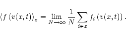
Let us consider a 1D stochastic time-dependent process v(x,t). A mean value of some function f(v) at position x and time t is computed from an ensemble $\varepsilon$ of N realisations of the process by:

$\begin{displaymath}\left\langle f\left( v(x,t\right) \right\rangle _{\varepsilon... ...\frac{1}{N}\sum _{i\in \varepsilon }f_{i}\left( v(x,t)\right). \end{displaymath}$

However, effective computation of that quantity requires discretisation of all variables. So let us choose a time step $\Delta t$ , a spatial step $\Delta x$ , and elementary step for variable v: $\Delta v$ . Then the indicatrix function ${\rm I\!I}^{v_{0}}_{x_{0},t_{0}}(v)$ is defined by: ${\rm I\!I}^{v_{0}}_{x_{0},t_{0}}(v)=1$ if $v_{0}\leq v<v_{0}+\Delta v$ where $x_{0}\leq x<x_{0}+\Delta x$ and $t_{0}\leq t<t_{0}+\Delta t$ ; and is zero anywhere else. Then we may write our definition of a mean value as:

$\begin{displaymath}\begin{array}{l} \left\langle f\left( v(x_{0},t_{0})\right) ... ...\varepsilon }~ {\rm I\!I}^{v}_{x_{0},t_{0}}\right) \end{array}\end{displaymath}$

where the sums extend over all possible values of v', xand t. The sum over all possible realisations now defines the probability distribution function of v, at x₀,t₀with resolution $\Delta x$ , $\Delta v$ . We write it P_x₀,t₀(v)or only P(v) hereafter.

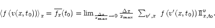
For one specific realisation $\varepsilon _{0}$ , we can also write a space mean of f(v) at given time t₀ as:

$\begin{displaymath}\begin{array}{l} \left\langle f\left( v(x,t_{0})\right) \righ... ...\left( v'(x,t_{0})\right) {\rm I\!I}^{v}_{x,t_{0}}. \end{array}\end{displaymath}$

The sum over v' and the indicatrix select the proper value of v at x.

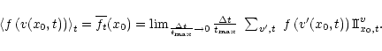
A time mean of f(v) at a given place x₀ is defined as:

$\begin{displaymath}\begin{array}{l} \left\langle f\left( v(x_{0},t)\right) \righ... ...\left( v'(x_{0},t)\right) {\rm I\!I}^{v}_{x_{0},t}. \end{array}\end{displaymath}$

Now, if the stochastic process v is homogeneous in space and stationary in time, then $\overline{f_{\varepsilon }}$ does not depend on x₀ (homogeneity) or on t₀ (stationarity). The latter hypothesis requires that our process be dissipative and that any initial condition be forgotten, that is $t_{\max }$ should be large compared to all characteristic time scales of the process. By the same argument, $\overline{f_{x}}$ does not depend on t₀, and $\overline{f_{t}}$ does not depend on x₀.

That these three mean values are the same follows Birkhoff's ergodic theorem, as developed in Frisch (1995) Chapters 3 and 4. Therefore, we get $\overline{f_{x}}=\overline{f_{t}}$ , which is the Taylor hypothesis.

If v is a 3D phenomenon, then isotropy is further required to chose at random a direction x so that the result is independent of that specific direction. Note that the argument does not depend on the choice of f, which can be any function of the stochastic process v, thus it is true for all moments of the process vitself, whatever its distribution function (Gaussian or not Gaussian).

Stationary developed turbulence is supposed to be homogeneous and isotropic so that this result applies for any component of the velocity field.

A.2 Extended Taylor hypothesis

Now let us consider a 2D stochastic process v. Using isotropy, we select a random direction x to which y is orthogonal. Then, we choose a segment S_y₀ along x at y₀. Again, space is discretised by $\Delta x=\Delta y$ , time by $\Delta t$ , and v (assumed scalar) by $\Delta v$ . All previous results apply to any one-point function of v, that is any mean quantity is independent of the choice of y₀ (homogeneity), of any x₀ along S_y₀ (homogeneity again), of time (stationarity) or of the choice of the initial direction (isotropy).

However, we may also define on S_y₀ two-point (or more) functions that are not taken care of by the previous results. For two points x₁ and x₂ along S_y₀ such that $\left\vert x_{2}-x_{1}\right\vert =L$ , we have:

$\begin{displaymath}\begin{array}{l} \left\langle f\left( v_{1}(x_{1},t_{0}),v_{2... ...I\!I}^{v_{1}}_{x,t_{0}}{\rm I\!I}^{v_{2}}_{x,t_{0}} \end{array}\end{displaymath}$

and an analogous expression for $\overline{f_{t}}(L)$ . But now, if L is shorter than any spatial correlation length of the process v, then the expression for $\overline{f_{x}}(L)$ does not factorise, since events at x₁ and x₂are not independent. However, it remains independent of y₀, x₁ and x₂ separately, and t₀. Only the distance L between the two points matters. By the same argument, $\overline{f_{t}}(L)$ is also independent of y₀, and x₁ and x₂ separately. We may again apply Birkhoff's theorem, and state that $\overline{f_{x}}(L)=\overline{f_{t}}(L)$ .

Strictly speaking, a third mean value can be defined, which is $\overline{f_{y}}(L)$ , for two points separated by L along direction x, but with samples taken out of parallel segments S_y along y. For a scalar process, isotropy ensures that $\overline{f_{x}}(L)=\overline{f_{y}}(L)$ . We assume here that the same is true for any component of the velocity field, thus neglecting the possible effect of cross-correlations.

Within that restriction, we see that, providing all sizes considered are large with respect to the largest correlation size within our sample, the same reasoning leads to a value of $\overline{f}(L)$ independent of the fact that we computed a spatial mean, or a temporal mean (in the same way that we needed to consider time scales large with respect to the largest correlation time to get the usual Taylor hypothesis). This is again independent of the choice of the function f and can be generalised to any number of points (or any order).

Thus we see that statistical properties of v along a segment S as time flows are the same as the statistical properties of a family of parallel segments in space at a given time. By choosing a "scanning velocity'' u₀, we are able to transform a 2D static field v(x,y) into a 1D, time varying field v(x,t=y/u₀).

Up: Interstellar turbulent velocity fields: chemistry