A&A 389, 1055-1067 (2002)
DOI: 10.1051/0004-6361:20020613
N. Décamp - J. Le Bourlot
LUTH, Observatoire de Paris et Université Paris 7, France
Received 26 November 2001 / Accepted 3 April 2002
Abstract
Turbulence is thought to play a key role in the dynamics of interstellar
clouds. Here, we do not seek to explain its origin or decipher the
mechanisms that maintain it, but we start from the observational fact
that it is present. Arnéodo et al. have developped a method based
on wavelet analysis to study incompressible turbulence experiments. We
propose to use this method with the same propagator to derive quantitative
information on the structure of a turbulent field. Then we build a
synthetic velocity field with the same statistical properties and
we show that a reactive fluid subject to turbulent forcing exhibits
self-organised structures that depend on the chemical species considered.
Such effects could explain why observational evidence shows that the
bulk of the mass is distributed smoothly whereas some chemical species
are extremely patchy.
Key words: turbulence - methods: numerical - ISM: general - ISM: molecules - ISM: structure
Turbulence has been believed to play a key role in the dynamics of molecular clouds for a long time (see for example Larson 1981; Myers 1983; Scalo 1987; Scalo 1990; Falgarone & Phillips 1990; Falgarone et al. 1994; Ballesteros-P. et al. 1999; Pety & Falgarone 2000). However, many questions are still subject to debate. What is the origin of that turbulence? Is compressibility an essential feature? What is the role of the magnetic field (e.g. Myers & Khersonsky 1995)? How does the velocity field couple to other aspects of interstellar cloud dynamics? The origin of these difficulties can be traced to at least two facts:
Progress has been made recently along two lines. Lis et al. (1996), Lis et al. (1998), Miesch & Scalo (1995) and
Miesch et al. (1999) have analysed the Probability Distribution Functions (PDF)
of line centroid velocity increments (see Appendix B).
These quantities are the closest available to velocity increment PDFs
widely used in laboratory experiments on turbulence (see Frisch 1995,
for the necessary background). These PDFs suggest that intermittency
is present in the turbulent velocity field. However, their best maps
come from the ![]() Ophiuchi cloud which exhibits an active
star formation region, and it is not clear whether the velocity field
is characteristic of turbulence alone or dominated by the interactions
between newly-formed YSOs and the embedding gas. Statistical analyses
have also been carried out, for example by Padoan et al. (1999).
Ophiuchi cloud which exhibits an active
star formation region, and it is not clear whether the velocity field
is characteristic of turbulence alone or dominated by the interactions
between newly-formed YSOs and the embedding gas. Statistical analyses
have also been carried out, for example by Padoan et al. (1999).
Although starting with very different assumptions, Stutzki et al. (1998) and Mac Low & Ossenkopf (2000) developed an analysis based on a form of wavelet transform (either directly or via some related mathematical tools). They have shown that quantitative information can be extracted in that way, but their results are plagued by a low signal-to-noise ratio and a lack of scale dynamics, which leads to heavy uncertainties. Furthermore, it is far from obvious how to use these results in order to gain a deeper understanding of the underlying physics.
Whatever the detailed characteristics of the velocity field inside
a molecular cloud, its influence on the dynamics of the gas and thus
on the interpretation of observational quantities has to be taken
into account. The first and most obvious effect is the interpretation
of line width as Doppler broadening. This gives a simple measure of
a typical velocity dispersion within the emitting region. In quiescent
clouds, that value is usually much higher than the pure thermal broadening
and controls the radiative cooling of the gas. There is now a fairly
well-established relation between velocity dispersion and the size
of the emitting region (
![]() ,
with
,
with
![]() (see e.g. Miesch & Bally 1994)). Evidence of high clumpiness
of the cloud density, or even of fractal structure may be found e.g.
in Falgarone et al. (1991) or Falgarone et al. (1994) and references therein.
(see e.g. Miesch & Bally 1994)). Evidence of high clumpiness
of the cloud density, or even of fractal structure may be found e.g.
in Falgarone et al. (1991) or Falgarone et al. (1994) and references therein.
An elaborate analysis of the interaction between line formation and a turbulent velocity field is given by Kegel et al. (1993) and Piehler & Kegel (1995) who compute the effects of a finite correlation length within a cloud (see also Park & Hong 1995). These computations prove that line profiles may be significantly modified and that neither micro- nor macro-turbulence approximations are usually valid. However, their cloud models are far too simple to take into account the real structure of a cloud and their mean field approach neglects realisation effects in any specific object. The latter point has been stressed by Rousseau et al. (1998), but their model is otherwise too qualitative and remote from observational aspects to shed much light on the physics of "real'' clouds.
Another potentially important influence of turbulence is on the chemical
evolution of molecular clouds. A number of key chemical species have
observational abundances far larger than what any model predicts.
The best case is that of
![]() whose only formation
route requires an energy of 4640 K, and is widely observed.
Intermittent dissipation of turbulence has been proposed as the source
of heat that could drive the formation. Since that dissipation occurs
in a small fraction of volume (typically less than 10-3),
the overall gas temperature is not affected. Joulain et al. (1998) have proposed
a model of chemistry within one specific vortex that supports well
that mechanism. Following Falgarone & Puget (1995), turbulence may also induce a
decoupling between gas and grains that leads to a high relative velocity
of the two fluids. The kinetic energy released in a gas-grain collision
then exceeds the thermal one and could help to drive slightly endothermic
reactions or increase collisional excitation.
whose only formation
route requires an energy of 4640 K, and is widely observed.
Intermittent dissipation of turbulence has been proposed as the source
of heat that could drive the formation. Since that dissipation occurs
in a small fraction of volume (typically less than 10-3),
the overall gas temperature is not affected. Joulain et al. (1998) have proposed
a model of chemistry within one specific vortex that supports well
that mechanism. Following Falgarone & Puget (1995), turbulence may also induce a
decoupling between gas and grains that leads to a high relative velocity
of the two fluids. The kinetic energy released in a gas-grain collision
then exceeds the thermal one and could help to drive slightly endothermic
reactions or increase collisional excitation.
It can be seen that the induced effects of a turbulent velocity field do not rely upon the fact that interstellar turbulence complies with what is implied by a canonical academic description of turbulence in fluids. Most phenomena follow only from the existence of a large deviation to from a Gaussian distribution of some properties of the velocity field (not necessarily the velocity components themselves). Therefore, in an attempt to study those effects, we do not need to solve the Navier-Stokes equations at a high Reynolds number in a compressible gas in order to build a realistic velocity field. Such a task is out of reach of present computing facilities, and even if achieved would leave no computing power to deal with chemistry, radiative transfer, and other intensive computing tasks. What we need is a velocity field compatible with all (or most) observational constraints. Then, once that field is built and characterised, it can be used as an input for a model of molecular clouds, and the effects of varying the velocity field measured in the model.
In this paper, we have tried to follow such a program (or at least the first steps of it). Current work on incompressible turbulence in the laboratory leads us to believe that the intrinsically multi-scale character of turbulence can only be grasped with a specifically multi-scale tool, namely wavelet transform.
In Sect. 2, we gather observational data and submit them to an analysis that extracts a small number of parameters that quantify interstellar turbulence under the assumption that results on incompressible terrestrial turbulence can be extended to compressible interstellar turbulence. In Sect. 3, we use these parameters to build a synthetic velocity field whose statistical properties are identical to the observed ones. In Sect. 4 we build a 1D time-dependent lattice dynamical network that is the frame on which our interstellar cloud model is built. In Sect. 5 we present a toy model chemistry with some qualitative properties of interstellar chemistry. In Sect. 6 that chemistry is coupled to the velocity field, and the structures that follow are illustrated. Section 7 is our conclusion.
Following Stutzki et al. (1998) we use a wavelet analysis to characterise
the velocity field in one specific interstellar cloud. However, the
particular method we chose is dictated by our reconstruction technique,
described below. The observational map has been collected during the
IRAM key project![]() , see Falgarone et al. (1998). It is a
, see Falgarone et al. (1998). It is a
![]() fully sampled
fully sampled
![]() map of the Polaris cloud. The pixel
size is 1125 AU for a cloud at 150 pc from the sun, and the
spectral resolution is
map of the Polaris cloud. The pixel
size is 1125 AU for a cloud at 150 pc from the sun, and the
spectral resolution is
![]() .
At each point
in the map, the centroid velocity was computed by J. Pety as described
in Lis et al. (1996) or Pety (1999) and kindly provided prior to publication
(Pety & Falgarone submitted). Note that these centroid velocity increments might differ
from the actual PDF of velocity differences due to various effects
such as radiative transfert effects or line of sight averaging.
.
At each point
in the map, the centroid velocity was computed by J. Pety as described
in Lis et al. (1996) or Pety (1999) and kindly provided prior to publication
(Pety & Falgarone submitted). Note that these centroid velocity increments might differ
from the actual PDF of velocity differences due to various effects
such as radiative transfert effects or line of sight averaging.
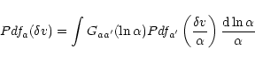
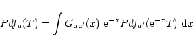
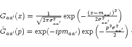
The method we use to build a velocity field takes into account that
turbulence is believed (at least in the inertial range) to be a multiplicative
cascade process. We follow the work of Castaing (1996) as extended by
Arnéodo et al. (1997), Arnéodo et al. (1998), Arnéodo et al. (1999). The basic concept is that the
PDF of velocity increments at one scale (a) can be expressed
as a weighted sum of dilated PDFs at a larger scale (a):
Arnéodo and collaborators have generalised this approach by computing
first the wavelet transform of the velocity field v. The PDFs
of the wavelet coefficients T (Pdf(T)) follow a relation
similar to that in Eq. (1), but here the propagator
is easily computed, allowing for a reconstruction of the velocity
field. Replacing ![]() by T and
by T and ![]() by e-x, Eq. (1) may be written:
by e-x, Eq. (1) may be written:
![\begin{figure}
\includegraphics[width=8.8cm,clip]{MS2137f1.eps}
\end{figure}](/articles/aa/full/2002/27/aa2137/img27.gif) |
Figure 1:
PDF of the velocity increments' absolute value
logarithm.
|
| Open with DEXTER | |
![\begin{figure}
\par\includegraphics[width=8.8cm,clip]{MS2137f2.eps}
\end{figure}](/articles/aa/full/2002/27/aa2137/img28.gif) |
Figure 2:
PDF of the wavelet coefficients' absolute value
logarithm.
|
| Open with DEXTER | |
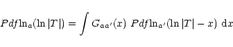
Using J. Pety's centroids of Polaris, Fig. 1 shows
the PDFs of
![]() ,
with
,
with
![]() and v(x)) the centroid velocity
at point x, for various scales a. Despite the rather
large size of our map, the PDFs are noisy. However, the evolution
through scales of the general shape is fairly regular.
and v(x)) the centroid velocity
at point x, for various scales a. Despite the rather
large size of our map, the PDFs are noisy. However, the evolution
through scales of the general shape is fairly regular.
Figure 2 shows the same analysis for the wavelet
coefficients![]() . We use a Daubechies 3 wavelet, which has a compact support in order
to minimise boundary effects. Order 3 is a compromise in order to
maintain enough regularity within our limited range of scales. Note
that order 1 would be equivalent to the previous velocity increments.
Increasing the order helps to eliminate large-scale effects in the
velocity field, but fewer ranges are accessible due to the larger
support requirement.
. We use a Daubechies 3 wavelet, which has a compact support in order
to minimise boundary effects. Order 3 is a compromise in order to
maintain enough regularity within our limited range of scales. Note
that order 1 would be equivalent to the previous velocity increments.
Increasing the order helps to eliminate large-scale effects in the
velocity field, but fewer ranges are accessible due to the larger
support requirement.
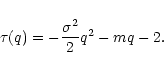
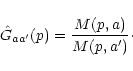
Assuming as above that the propagator is Gaussian, we may write:
The evolution of the propagator parameters versus the logarithm of
the scales ratio (Fig. 3) is linear within the error
bars which suggests a second assumption: the cascade is scale-similar
(or scale-invariant). This means that
![]() for
a'>a and leads to
for
a'>a and leads to
![]() and
and
![]() .
Actually, as developped in Arnéodo et al. (1998) the scale similarity is a specific
case of continuously self-similar cascades that have a propagator
satisfying the following relation:
.
Actually, as developped in Arnéodo et al. (1998) the scale similarity is a specific
case of continuously self-similar cascades that have a propagator
satisfying the following relation:
![]() where
s(a,a')=s(a')-s(a). The function s(a) could have
the following form:
where
s(a,a')=s(a')-s(a). The function s(a) could have
the following form:
![]() with a very
small value for
with a very
small value for ![]() ;
the small range of scales in our study
prevents us from distinguishing between this form and
;
the small range of scales in our study
prevents us from distinguishing between this form and ![]() (scale similarity). In both cases, we find values of m and
(scale similarity). In both cases, we find values of m and
![]() of:
of:
![]() and
and
![]() .
These values are used in the following sections.
.
These values are used in the following sections.
![\begin{figure}
\includegraphics[angle=270,width=8.8cm,clip]{MS2137f3a.eps}\par\includegraphics[angle=270,width=8.8cm,clip]{MS2137f3b.eps}
\end{figure}](/articles/aa/full/2002/27/aa2137/img43.gif) |
Figure 3:
Mean and standard deviation of the propagator
versus scale difference.
|
| Open with DEXTER | |
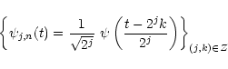
We generate a velocity field by constructing its wavelet decomposition
coefficients. We use the concept of multi-resolution associated with
an orthogonal wavelet (see Mallat 1999): the dilated and translated
family
The standard deviation of the velocity field as a function of size
is plotted in Fig. 4. The law
![]() fits
both the synthetic velocity field and the Polaris region well with
an exponent of
fits
both the synthetic velocity field and the Polaris region well with
an exponent of
![]() in both cases. This exponent
is clearly irrelevant (or equal to 0) for a classical Gaussian field:
for such a field the standard deviation is the same for any scale;
the difference observed is just a sampling effect. The model is adjusted
to observations by fixing d0,0 so that the curves coincide.
Here,
d0,0=250 for 13 octaves (reductions of scale by a
factor of 2) between the integral scale and the
in both cases. This exponent
is clearly irrelevant (or equal to 0) for a classical Gaussian field:
for such a field the standard deviation is the same for any scale;
the difference observed is just a sampling effect. The model is adjusted
to observations by fixing d0,0 so that the curves coincide.
Here,
d0,0=250 for 13 octaves (reductions of scale by a
factor of 2) between the integral scale and the ![]() scale.
scale.
The resulting velocity field is then submitted to the same analysis
as the original one, and the number of steps between our integral
scale and the Polaris map scale is fixed by adjusting the non-Gaussian
wings. Figure 5 shows the resulting PDFs. Here N=13between the integral scale and the ![]() scale. Note that
the synthetic field PDFs are in good agreement with the observed ones,
and that the synthetic field is correlated at all scales (a rough
estimate of the synthetic signal correlation length at scale ais a) unlike the uncorrelated Gaussian field used for comparisons.
scale. Note that
the synthetic field PDFs are in good agreement with the observed ones,
and that the synthetic field is correlated at all scales (a rough
estimate of the synthetic signal correlation length at scale ais a) unlike the uncorrelated Gaussian field used for comparisons.
We are now able to determine the scaling of our model by identifying
size at scale N with Polaris resolution. In Fig. 5,
![]() pixels corresponds to
lN=2250 AU, so that
our integral scale is
pixels corresponds to
lN=2250 AU, so that
our integral scale is
![]() .
Note that this is not the size of the cloud that we generate: the
Polaris map size is reached after 9 steps in the generating process.
A side effect of that sub-sampling is that the mean global velocity
of the generated cloud is slightly non 0.0 (see Sect. 4.4).
.
Note that this is not the size of the cloud that we generate: the
Polaris map size is reached after 9 steps in the generating process.
A side effect of that sub-sampling is that the mean global velocity
of the generated cloud is slightly non 0.0 (see Sect. 4.4).
![\begin{figure}
\par\includegraphics[width=8.8cm,clip]{MS2137f4.eps}
\end{figure}](/articles/aa/full/2002/27/aa2137/img60.gif) |
Figure 4:
Standard deviation of the velocity field as a function
of size l (in pixel units) for Polaris, for the synthetic field, and
for a Gaussian field. The vertical offset of the model is fixed by
|
| Open with DEXTER | |
![\begin{figure}
\includegraphics[width=8.8cm,clip]{MS2137f5r.eps}
\end{figure}](/articles/aa/full/2002/27/aa2137/img61.gif) |
Figure 5: Comparison between the velocity increments' PDFs of the Polaris map (points) and the reconstructed field (lines) for different scales. |
| Open with DEXTER | |
The use of a wavelet decomposition of our synthetic velocity field
gives access to the best approximation at any scale between the integral
scale l0 (where it is just the mean velocity, and is 0.0by construction) and the smallest accessible scale
![]() ,
where
,
where ![]() is the number of steps in the wavelet transform.
is the number of steps in the wavelet transform.
As we are interested in the effects of turbulence on the dynamics
of a cloud, the smallest significant scale is the turbulence dissipation
length. Any cell of gas smaller than that length is homogeneous and
statistically identical to its nearest neighbour. That scale may be
estimated from classical results on Kolmogorov turbulence (see Frisch 1995):
the energy flux through scales is
![]() ,
which is true also at lN, the Polaris resolution scale with
vN, the turbulent velocity at that scale. We can estimate
that quantity from the observations if we take
,
which is true also at lN, the Polaris resolution scale with
vN, the turbulent velocity at that scale. We can estimate
that quantity from the observations if we take ![]() ,
the
standard deviation of centroids increments at scale lN,
as an estimate of vN. From the Polaris map,
,
the
standard deviation of centroids increments at scale lN,
as an estimate of vN. From the Polaris map,
![]() ,
so that
,
so that
![]() .
Then
the dissipation scale is given by
.
Then
the dissipation scale is given by
![]() ,
where
,
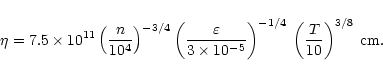
where ![]() is the kinematic viscosity. In a diluted gas,
is the kinematic viscosity. In a diluted gas,
![]() ,
where
,
where
![]() is the thermal velocity, n the gas density,
and
is the thermal velocity, n the gas density,
and ![]() the collision cross section. Inside a molecular
gas, we can take a mean
the collision cross section. Inside a molecular
gas, we can take a mean
![]() -
-
![]() cross section
of
cross section
of
![]() (see Le Bourlot et al. (1999)),
a density of
(see Le Bourlot et al. (1999)),
a density of
![]() and a temperature of
and a temperature of
![]() .
This gives:
.
This gives:
Since we are not interested in the physics inside that box, we can
use a coarse-grained approximation by looking at a collection of identical
cells of size
![]() ,
coupled by convection (hence our
need to prescribe the velocity field) or radiatively (i.e. in velocity
space nearest neighbour but not necessarily in physical space, see
Rousseau et al. 1998). Thus, we by-pass the need to solve partial differential
equations and need only to prescribe the evolution of mean variables
inside each box and their mutual coupling (hereafter only by convection).
The most accurate way to realise that smoothing is to use the approximation
coefficients of the wavelet transform at that scale.
,
coupled by convection (hence our
need to prescribe the velocity field) or radiatively (i.e. in velocity
space nearest neighbour but not necessarily in physical space, see
Rousseau et al. 1998). Thus, we by-pass the need to solve partial differential
equations and need only to prescribe the evolution of mean variables
inside each box and their mutual coupling (hereafter only by convection).
The most accurate way to realise that smoothing is to use the approximation
coefficients of the wavelet transform at that scale.
So we consider a set of identical boxes, each characterised by local
dynamics (a set of local variables, coupled by physical relationships)
with the same variables and evolution laws in each cell, but not necessarily
the same initial conditions. Evolution is computed over a continuous
time within each box, and a spatial coupling is applied at discrete
times. The velocity at the smallest scale
![]() is taken
as the mean velocity of a box in a rest frame. Therefore we use an
Eulerian representation. Velocity is prescribed a priori, and is not
modified by the evolution of any local variable. It is understood
that the way the velocity field is built takes care of all (mostly
unknown) processes that constrain its evolution. What we need now
is a way to progress in time.
is taken
as the mean velocity of a box in a rest frame. Therefore we use an
Eulerian representation. Velocity is prescribed a priori, and is not
modified by the evolution of any local variable. It is understood
that the way the velocity field is built takes care of all (mostly
unknown) processes that constrain its evolution. What we need now
is a way to progress in time.
As a first stage, our goal is to model a cloud in steady state. This means that all its statistical properties remain constant on average, but are not necessarily time independent! They may fluctuate in time around a mean value, and only that value is constant in time. This has to be true also for the velocity field, so that we need to prescribe the evolution in time of the static field of Sect. 3. To that end, we make the hypothesis that turbulence is homogeneous, isotropic, and stationary. Under these three conditions, the Taylor hypothesis applies and the statistical properties of v(x0,t) as t varies are the same as those of v(x,t0) along an axis x. This hypothesis may be extended to a 1D structure: the statistical properties of a velocity field v(X,t) along an axis X as t varies are the same as that of a collection of lines in a 2D plane at a given time t0. The second hypothesis is stronger than the first because cross-correlations between orthogonal directions X and Y have to be included and is only true if the three conditions of homogeneity, isotropy, and stationarity strictly apply, see Appendix A for a demonstration.
The extension to 2D of the velocity field generation algorithm is
straightforward (although computationally intensive). Details are
given in Arnéodo et al. (1999) and references therein (see Appendix C).
Once a 2D X-Y field has been generated, the Y axis can
be interpreted as u0t, where u0 is a "scanning''
velocity that sets a time scale for the model. For consistency, we
take
![]() .
From this point, the velocity in
our model is prescribed in each box of size
.
From this point, the velocity in
our model is prescribed in each box of size
![]() and at each time
and at each time
![]() (where
(where
![]() is the crossing
time at the smallest scale).
is the crossing
time at the smallest scale).
Mass conservation reads:
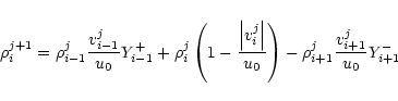
We use uniform initial conditions and assume periodic boundary conditions.
Equation (10) is solved in each "box'' as a balance
equation. We "count'' the total amount of matter that escapes
and enters each box: namely, for three successive boxes (at step j,
density
![]() ,
,
![]() and
and
![]() and velocity
vji-1, vji and
vji+1,
we have:
and velocity
vji-1, vji and
vji+1,
we have:
![\begin{figure}
\includegraphics[width=8.8cm,clip]{MS2137f6.eps}
\end{figure}](/articles/aa/full/2002/27/aa2137/img97.gif) |
Figure 6: Relative difference (in %) in the standard deviation of the density field as a function of time for two different initial fields (constant initial density of 1 and random initial density in the range [0; 2]). |
| Open with DEXTER | |
After a transitory period, the density and velocity fields "couple'' together and the standard deviation stabilises (the mean density is constant because periodic boundary conditions ensure conservation of the total mass). In Fig. 6 we have plotted the evolution (after the transitory period) of the relative difference in the standard deviation for two different initial density fields (random value on the interval [0; 2] and a constant initial density of 1): this relative difference maintains a very small value (typically 1%).
A typical example of a density field is given in the top panel of
Fig. 7. We see that large fluctuations of ![]() are possible within a few cells and dense cores develop over a low-density
background.
are possible within a few cells and dense cores develop over a low-density
background.
The density field obtained with our synthetic turbulent velocity field
and the one obtained with a Gaussian velocity field of the same mean
and standard deviation are very different (see Fig. 7):
for the Gaussian field, the density seems relatively uniform but for
the turbulent field, some structures appear naturally at all scales. Figure 8
shows the PDF of the logarithm of the density obtained with our synthetic
turbulent velocity field. It is log-normal towards high density and
exhibits a strong power law towards low density. The high density
cut-off is a finite size effect, and the power law may be interpreted
as an indication that our velocity field mimics that of a non-isothermal
fluid, but we did not try to check that point further. This point
will be dealt with in a further paper with an improved model, easier
to compare to observations and hydrodynamical models.
![\begin{figure}
\includegraphics[width=8.8cm,clip]{MS2137f7a.eps}\par\includegraphics[width=8.8cm,clip]{MS2137f7b.eps}
\end{figure}](/articles/aa/full/2002/27/aa2137/img99.gif) |
Figure 7: Log of the density field for a turbulent and for a Gaussian velocity field (mean and standard deviation are the same for both fields). |
| Open with DEXTER | |
![\begin{figure}
\includegraphics[angle=270,width=8.8cm,clip]{MS2137f8.eps}
\end{figure}](/articles/aa/full/2002/27/aa2137/img100.gif) |
Figure 8: Pdf of the logarithm of the density for our turbulent velocity field. |
| Open with DEXTER | |
A relation between size and density can be computed: Using a Gaussian
wavelet we compute for each scale the mean value of the density above
the mean (which is here the same at all scales). Figure 9
shows a power law relation with an index of
![]() .
This is much lower than the
.
This is much lower than the
![]() law
that results from self-gravitating clouds. Such a flat index is probably
a consequence of our 1D model and further discussions should wait
for 2D results.
law
that results from self-gravitating clouds. Such a flat index is probably
a consequence of our 1D model and further discussions should wait
for 2D results.
![\begin{figure}
\includegraphics[width=8.8cm,clip]{MS2137f9.eps}
\end{figure}](/articles/aa/full/2002/27/aa2137/img103.gif) |
Figure 9: Decimal logarithm of the density as a function of scale. |
| Open with DEXTER | |
Mixing properties of our synthetic velocity field may be derived from the evolution in time of the distribution of a passive scalar (say a non-reacting chemical species). The initial density is 1 in a single box located at x=256 and 0 elsewhere. The density after 1024 iterations (i.e. some 17 Myr) is shown Fig. 10 for two different velocity fields: a random Gaussian field (without correlations), and our synthetic turbulent field.
The resulting density profiles are quite different: a random Gaussian
field leads to a localised Gaussian profile, whilst a turbulent field
leads to a wider dispersion after a much shorter time (typically,
the large-scale turnover time, here, about 1 Myr). As a check of our
numerical procedure, we plot in Fig. 11 the mean
position (relative to the initial maximum position) and standard deviation
of the density profile obtained with the Gaussian velocity field.
As expected, the mean position is a linear function of time (
![]() ,
here
,
here
![]() and the fit gives
and the fit gives
![]() )
and the standard deviation
increases as the square root of time (
)
and the standard deviation
increases as the square root of time (
![]() with the diffusion coefficient
with the diffusion coefficient
![]() ,
here
,
here
![]() and the result
of the fit is 0.76). These results demonstrate that our lattice
dynamical network is an accurate approximation of the diffusion equation.
and the result
of the fit is 0.76). These results demonstrate that our lattice
dynamical network is an accurate approximation of the diffusion equation.
Interstellar chemistry is known to be sensitive to density since some destruction processes (photo-ionisation and/or destruction by cosmic rays) proceed as the density, whereas chemical reactions proceed as the square of the density. Le Bourlot et al. (1995) have shown that under some fairly ordinary physical conditions, two stable chemical phases may exist. So, depending on initial conditions, some parts of the cloud may evolve towards one phase as others evolve towards the other phase. Interfaces between those phases lead to reaction-diffusion fronts where unusual chemical abundances may prevail for long times in a manner similar to reaction-diffusion fronts in a thermally bistable fluid studied by Shaviv & Regev (1994).
Thus, a minimal local dynamic should at least exhibit bistability.
This can be achieved with a 3-variable model which is the minimal
non-passive scalar model possible. By turning on or off turbulent
mixing, we can test the effects of that mixing on mean abundances
along the line of sight and on time and length scales for each variable
within the cloud.
![\begin{figure}
\par\includegraphics[width=8.8cm,clip]{MS2137f10.eps}
\end{figure}](/articles/aa/full/2002/27/aa2137/img111.gif) |
Figure 10:
Dispersion of a passive scalar (after 1024 iterations of
|
| Open with DEXTER | |
![\begin{figure}
\includegraphics[angle=270,width=6.8cm,clip]{MS2137f11a.eps}\par\includegraphics[angle=270,width=6.8cm,clip]{MS2137f11b.eps}
\end{figure}](/articles/aa/full/2002/27/aa2137/img112.gif) |
Figure 11: Temporal evolution of the mean and standard deviation of the passive scalar density distribution for our two fields. As expected for diffusion by a Gaussian field, the mean and variance are proportional to time. |
| Open with DEXTER | |
This is an extension to intrinsically scale-dependent models of the work of Xie et al. (1995) and Chièze & Des Forêts (1989). However, full-size interstellar chemical schemes are still beyond our reach.
As a test model, we chose the following set of chemical reactions
(inspired from Gray & Scott 1990):
If we suppose that k1 has the following temperature dependence
![]() and that reaction
(4) is exothermic, then thermal balance is governed by:
and that reaction
(4) is exothermic, then thermal balance is governed by:
![]() (with
(with
![]() ). Here the cooling
term mimics radiative cooling by both A and B after
collisional excitation.
). Here the cooling
term mimics radiative cooling by both A and B after
collisional excitation.
We can reduce the problem to a simple dynamical system with three
differential equations and four parameters
![]() :
:
![\begin{figure}
\includegraphics[width=6.8cm,clip]{MS2137f12a.eps}\par\includegraphics[width=6.8cm,clip]{MS2137f12br.eps}
\end{figure}](/articles/aa/full/2002/27/aa2137/img126.gif) |
Figure 12:
An example of bistability and limit cycle
with Hopf bifurcation. The parameters values are
|
| Open with DEXTER | |
It is then possible to add the effects of that non-trivial local dynamic
to turbulent mixing. We select the model of Sect. 5.
In order to study the influence of the turbulence, we again do a comparison
between a turbulent and a Gaussian velocity field (Fig. 13
for one example). Note that A, B (chemical species),
U (internal energy) and R (proportional to the total
density) are advected as described by Eq. (11) extended
to 4 variables.
![\begin{figure}
\par\includegraphics[width=6.8cm,clip]{MS2137f13a.eps}\par\includegraphics[width=6.8cm,clip]{MS2137f13b.eps}
\end{figure}](/articles/aa/full/2002/27/aa2137/img128.gif) |
Figure 13:
Density of component |
| Open with DEXTER | |
![\begin{figure}
\includegraphics[width=8.8cm,clip]{MS2137f14.eps}
\end{figure}](/articles/aa/full/2002/27/aa2137/img130.gif) |
Figure 14:
Density of components |
| Open with DEXTER | |
We can observe that, as in the previous case (Sect. 4.3), structures appear naturally at all scales in the turbulent case and not with a Gaussian velocity field. Appendix D shows the variations of A on a much larger time scale. Different initial conditions give indistinguishable results, suggesting that steady state is reached. However, we cannot exclude that some long time drift may still exist which our computation is unable to uncover.
Turbulent structures are not the same for the different components
(A, B, R) neither in position nor in size, as
can be seen in Fig. 14, which is an horizontal
cut of Fig. 13. In order to study more precisely
these effects, we plot the probability density function of A(Fig. 15) which should be compared to Fig 8.
![\begin{figure}
\includegraphics[width=8.8cm,clip]{MS2137f15.eps}
\end{figure}](/articles/aa/full/2002/27/aa2137/img131.gif) |
Figure 15:
Probability density function of |
| Open with DEXTER | |
Note that the presence of a non-uniform velocity field leads to a single-peaked broad distribution. Turbulence leads to a broader distribution and extended wings. Thus the probability to find some regions at far from equilibrium values is enhanced.
We also plotted the density of
![]() as a function of size (see Fig. 16) using the same
procedure as for Fig. 9. The slope is
as a function of size (see Fig. 16) using the same
procedure as for Fig. 9. The slope is
![]() (instead of
(instead of
![]() for the total density, cf. Sect. 4.3).
The evolution through scales is therefore significantly different
for one particular component and for the total density.
for the total density, cf. Sect. 4.3).
The evolution through scales is therefore significantly different
for one particular component and for the total density.
The structure of interstellar clouds remains a subject of debate because different observations suggest different, and often contradictory, interpretations. The Thoraval et al. (1999) results, based on infrared observations are sensitive mainly to the dust distribution and thus probably to the bulk of the mass distribution. On the contrary, some low-abundance species (see for example Marscher et al. 1993 and Moore & Marscher 1995 results) exhibit large abundance variations down to the smallest accessible scales.
Our results show that the structuring of the gas by the turbulent velocity field leads naturally to different distributions for different species, without requiring any external mechanism. Thus, seemingly contradictory observations find a unified explanation which applies to any turbulent region in the interstellar medium. Naturally, this does not preclude a significant influence of other mechanisms. Star formation does occur within clouds and leads to a number of fancy phenomena that stimulate the imagination of the modelist. We still need to explain how turbulence survives and is fed despite its fast dissipation timescale. However, since it is there, it must be taken into account.
In this paper, we have shown how interstellar turbulence properties
could be reduced to a small number of quantitative parameters by wavelet
analysis. A pure log-normal cascade (as in incompressible turbulence) is
characterised with only two numerical quantities. Deviation from that
behaviour could be managed with a third. These parameters are directly
accessible from observations, but require fully sampled, large-scale,
high-resolution maps. New observational facilities such as array detectors
now available at the 30 m IRAM observatory (HERA), or the future ALMA
project should provide such maps at a reasonable cost.
![\begin{figure}
\includegraphics[width=8.8cm,clip]{MS2137f16.eps}
\end{figure}](/articles/aa/full/2002/27/aa2137/img136.gif) |
Figure 16:
Decimal logarithm of
|
| Open with DEXTER | |
These parameters can be used to build synthetic velocity fields at a numerical cost well below that of solving the full Navier-Stokes equations. Time and length scales are easily adjusted to the observations, allowing for direct comparison of predicted and observed structures. Generalisation to 2D and 3D fields of techniques described here is straightforward, but would then require the use of large, massively parallel computers. It is not obvious that qualitatively different results would result from such an extension, with one exception: a 1D velocity field precludes vorticity and so our density field probably has excessive contrasts when matter is squeezed between two cells with opposite velocity direction. Extension of the chemical set is straightforward.
We have shown that a density structure develops with different scale properties for different chemical species. The mixing properties of turbulence ensure that on any line of sight a fraction of the gas is in a far from equilibrium state. Thus species that do not peak at the same evolutionary stage in a classical time-dependent model can coexist naturally without the need to invoke any "early-stage'' argument. Conversely no indication about the age of the cloud may be derived from abundance ratios.
Acknowledgements
We thank J. Pety for providing centroids map of Polaris prior to publication (Pety & Falgarone submitted, Pety 1999), D. Pelat for many discussions on subtle statistical matters, A. Arnéodo for discussions during a one week post-graduate course in Bordeaux, and E. Falgarone and the referee for numerous useful comments.
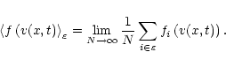
Let us consider a 1D stochastic time-dependent process v(x,t).
A mean value of some function f(v) at position x and
time t is computed from an ensemble
![]() of
N realisations of the process by:
of
N realisations of the process by:

For one specific realisation
![]() ,
we can also
write a space mean of f(v) at given time t0 as:
,
we can also
write a space mean of f(v) at given time t0 as:
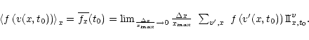
A time mean of f(v) at a given place x0 is defined
as:
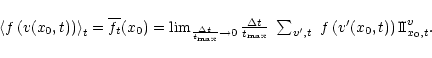
Now, if the stochastic process v is homogeneous in
space and stationary in time, then
![]() does not depend on x0 (homogeneity) or on t0 (stationarity).
The latter hypothesis requires that our process be dissipative and
that any initial condition be forgotten, that is
does not depend on x0 (homogeneity) or on t0 (stationarity).
The latter hypothesis requires that our process be dissipative and
that any initial condition be forgotten, that is ![]() should be large compared to all characteristic time scales of the
process. By the same argument,
should be large compared to all characteristic time scales of the
process. By the same argument,
![]() does not depend
on t0, and
does not depend
on t0, and
![]() does not depend on x0.
does not depend on x0.
That these three mean values are the same follows Birkhoff's ergodic
theorem, as developed in Frisch (1995) Chapters 3 and 4. Therefore, we
get
![]() ,
which is the Taylor
hypothesis.
,
which is the Taylor
hypothesis.
If v is a 3D phenomenon, then isotropy is further required to chose at random a direction x so that the result is independent of that specific direction. Note that the argument does not depend on the choice of f, which can be any function of the stochastic process v, thus it is true for all moments of the process vitself, whatever its distribution function (Gaussian or not Gaussian).
Stationary developed turbulence is supposed to be homogeneous and isotropic so that this result applies for any component of the velocity field.
However, we may also define on Sy0 two-point (or more)
functions that are not taken care of by the previous results. For
two points x1 and x2 along Sy0 such
that
![]() ,
we have:
,
we have:

Strictly speaking, a third mean value can be defined, which is
![]() ,
for two points separated by L along direction x, but
with samples taken out of parallel segments Sy along y.
For a scalar process, isotropy ensures that
,
for two points separated by L along direction x, but
with samples taken out of parallel segments Sy along y.
For a scalar process, isotropy ensures that
![]() .
We assume here that the same is true for any component of the velocity
field, thus neglecting the possible effect of cross-correlations.
.
We assume here that the same is true for any component of the velocity
field, thus neglecting the possible effect of cross-correlations.
Within that restriction, we see that, providing all sizes considered
are large with respect to the largest correlation size within our
sample, the same reasoning leads to a value of
![]() independent of the fact that we computed a spatial mean, or a temporal
mean (in the same way that we needed to consider time scales large
with respect to the largest correlation time to get the usual Taylor
hypothesis). This is again independent of the choice of the function
f and can be generalised to any number of points (or any order).
independent of the fact that we computed a spatial mean, or a temporal
mean (in the same way that we needed to consider time scales large
with respect to the largest correlation time to get the usual Taylor
hypothesis). This is again independent of the choice of the function
f and can be generalised to any number of points (or any order).
Thus we see that statistical properties of v along a segment S as time flows are the same as the statistical properties of a family of parallel segments in space at a given time. By choosing a "scanning velocity'' u0, we are able to transform a 2D static field v(x,y) into a 1D, time varying field v(x,t=y/u0).
The centroid velocity (C) is the mean radial velocity: if we
call T(u) the intensity as a function of the radial velocity,
then by definition
![]() .
In the case of an optically thin medium,
.
In the case of an optically thin medium,
![]() ,
where N(u) is the column density as a function of the radial
velocity (
,
where N(u) is the column density as a function of the radial
velocity (
![]() ). It is then easy to
show that
). It is then easy to
show that
![]() .
This
quantity is very commonly used because of the lack of information
about the velocity spatial repartition along the line of sight. The
centroid velocity increment at scale a is then:
.
This
quantity is very commonly used because of the lack of information
about the velocity spatial repartition along the line of sight. The
centroid velocity increment at scale a is then:
![]() ,
where r is a position on the plane of the sky. The probability
density function (PDF) of this quantity in a turbulent velocity field
is essentially indistinguishable from a Gaussian for the integral
scale and develops more and more non-Gaussian wings as the lag decrease
(see Lis et al. 1996; Pety 1999; Miesch et al. 1999).
,
where r is a position on the plane of the sky. The probability
density function (PDF) of this quantity in a turbulent velocity field
is essentially indistinguishable from a Gaussian for the integral
scale and develops more and more non-Gaussian wings as the lag decrease
(see Lis et al. 1996; Pety 1999; Miesch et al. 1999).
For any function
![]() ,
f can be written
under the form
,
f can be written
under the form
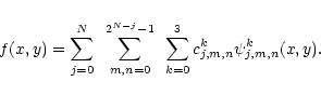
The wavelet coefficients themselves are computed via two angles
![]() :
:
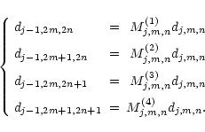
![\begin{displaymath}\left\{ \begin{array}{lcl}
c^{1}_{j,m,n} & = & \cos(\phi )\co...
...m]
c^{3}_{j,m,n} & = & \sin(\phi )d_{j,m,n}
\end{array}\right. \end{displaymath}](/articles/aa/full/2002/27/aa2137/img177.gif)
c10,0,0 = d0,0,0,
c20,0,0 = d0,0,0,
and
![]() (see Decoster et al. 2000 for all details).
(see Decoster et al. 2000 for all details).
We give in Figs. D.1 to D.4 the evolution
of the ![]() density with the same turbulent field and the
same parameters as in Fig. 13 but on a larger
time scale.
density with the same turbulent field and the
same parameters as in Fig. 13 but on a larger
time scale.
![\begin{figure}
\par\includegraphics[width=8cm,clip]{MS2137fD1.eps}\hspace*{4mm}\end{figure}](/articles/aa/full/2002/27/aa2137/img186.gif)
![\begin{figure}
\includegraphics[width=8cm,clip]{MS2137fD2.eps}
\end{figure}](/articles/aa/full/2002/27/aa2137/img187.gif)
![\begin{figure}
\includegraphics[width=8cm,clip]{MS2137fD3.eps}
\end{figure}](/articles/aa/full/2002/27/aa2137/img188.gif)
![\begin{figure}
\includegraphics[width=8cm,clip]{MS2137fD4.eps}
\end{figure}](/articles/aa/full/2002/27/aa2137/img189.gif)