A&A 389, 665-679 (2002)
DOI: 10.1051/0004-6361:20020596
T. G. Müller1,2 - S. Hotzel3 - M. Stickel3
1 - Max-Planck-Institut für extraterrestrische Physik,
Giessenbachstraße, 85748 Garching, Germany
2 -
ISO Data Centre, Astrophysics Division, Space Science
Department of ESA, Villafranca, PO Box 50727,
28080 Madrid, Spain (until Dec. 2001)
3 -
ISOPHOT Data Centre, Max-Planck-Institut für Astronomie,
Königstuhl 17, 69117 Heidelberg, Germany
Received 14 January 2002 / Accepted 12 March 2002
Abstract
The ISOPHOT Serendipity Survey (ISOSS) covered approximately 15%
of the sky at a wavelength of 170 ![]() m while the ISO satellite
was slewing from one target to the next. By chance, ISOSS slews
went over many solar system objects (SSOs). We identified
the comets, asteroids and planets in the slews through a fast
and effective search procedure based on N-body ephemeris and
flux estimates. The detections were analysed from a calibration and
scientific point of view.
Through the measurements of the well-known asteroids Ceres, Pallas,
Juno and Vesta and the planets Uranus and Neptune it was possible to
improve the photometric calibration of ISOSS and to extend it to
higher flux regimes. We were also able to establish calibration
schemes for the important slew end data.
For the other asteroids we derived radiometric diameters and albedos
through a recent thermophysical model. The scientific results
are discussed in the context of our current knowledge of
size, shape and albedos, derived from IRAS observations,
occultation measurements and lightcurve inversion techniques.
In all cases where IRAS observations were available we confirm
the derived diameters and albedos. For the five asteroids without
IRAS detections only one was clearly detected and the radiometric
results agreed with sizes given by occultation and HST observations.
Four different comets have clearly been detected at 170
m while the ISO satellite
was slewing from one target to the next. By chance, ISOSS slews
went over many solar system objects (SSOs). We identified
the comets, asteroids and planets in the slews through a fast
and effective search procedure based on N-body ephemeris and
flux estimates. The detections were analysed from a calibration and
scientific point of view.
Through the measurements of the well-known asteroids Ceres, Pallas,
Juno and Vesta and the planets Uranus and Neptune it was possible to
improve the photometric calibration of ISOSS and to extend it to
higher flux regimes. We were also able to establish calibration
schemes for the important slew end data.
For the other asteroids we derived radiometric diameters and albedos
through a recent thermophysical model. The scientific results
are discussed in the context of our current knowledge of
size, shape and albedos, derived from IRAS observations,
occultation measurements and lightcurve inversion techniques.
In all cases where IRAS observations were available we confirm
the derived diameters and albedos. For the five asteroids without
IRAS detections only one was clearly detected and the radiometric
results agreed with sizes given by occultation and HST observations.
Four different comets have clearly been detected at 170 ![]() m
and two have marginal detections. The observational results are
presented to be used by thermal comet models in the future.
The nine ISOSS slews over Hale-Bopp revealed extended
and asymmetric structures related to the dust tail. We attribute
the enhanced emission in post-perihelion observations to large
particles around the nucleus. The signal patterns are indicative of
a concentration of the particles in the trail direction.
m
and two have marginal detections. The observational results are
presented to be used by thermal comet models in the future.
The nine ISOSS slews over Hale-Bopp revealed extended
and asymmetric structures related to the dust tail. We attribute
the enhanced emission in post-perihelion observations to large
particles around the nucleus. The signal patterns are indicative of
a concentration of the particles in the trail direction.
Key words: minor planets, asteroids - comets: general - planets and satellites: general - infrared: solar system - surveys
The Infrared Space Observatory (ISO) (Kessler et al. 1996) made
during its lifetime between 1995 and 1998 more than 30 000 individual
observations, ranging from objects in our own solar system
right out to the most distant extragalactic sources. The solar
system programme consisted of many spectroscopic and photometric
studies of comets, asteroids, planets and their satellites at
near- and mid-infrared (near-/mid-IR) wavelengths
between 2.5 and 45 ![]() m. At far-infrared (far-IR) wavelengths,
beyond 45
m. At far-infrared (far-IR) wavelengths,
beyond 45 ![]() m, the programmes were limited to spectroscopic
observations of the outer planets, 3 satellites (Ganymede, Callisto,
Titan), 3 comets (P/Hale-Bopp, P/Kopff, P/Hartley 2) and 4 asteroids
(Ceres, Pallas, Vesta, Hygiea). Far-IR photometry on solar system
objects was mainly done for calibration purposes (Uranus, Neptune and
a few asteroids) and scientific studies of extended sources
(P/Hale-Bopp, P/Kopff, P/Wild 2, P/Schwassmann-Wachmann, Chiron, Pholus).
m, the programmes were limited to spectroscopic
observations of the outer planets, 3 satellites (Ganymede, Callisto,
Titan), 3 comets (P/Hale-Bopp, P/Kopff, P/Hartley 2) and 4 asteroids
(Ceres, Pallas, Vesta, Hygiea). Far-IR photometry on solar system
objects was mainly done for calibration purposes (Uranus, Neptune and
a few asteroids) and scientific studies of extended sources
(P/Hale-Bopp, P/Kopff, P/Wild 2, P/Schwassmann-Wachmann, Chiron, Pholus).
In addition to the dedicated programmes on individual sources, ISO
also made parallel and serendipitous observations of the sky. ISOCAM
observed the sky in parallel mode a few arc minutes away from the
primary target at wavelengths between 6 and 15 ![]() m (Siebenmorgen
et al. 2000). The ISOPHOT Serendipity Survey
(Bogun et al. 1996)
recorded the 170
m (Siebenmorgen
et al. 2000). The ISOPHOT Serendipity Survey
(Bogun et al. 1996)
recorded the 170 ![]() m sky brightness when the satellite was
slewing from one target to the next. LWS performed parallel
(Lim et al. 2000) and serendipitous surveys
(Vivarès et al. 2000) in the far-IR.
These complementary surveys contain many interesting objects, but the
scientific analysis only began recently. The two LWS surveys and the
ISOCAM parallel survey just underwent a first data processing and
could therefore not be considered in the following.
m sky brightness when the satellite was
slewing from one target to the next. LWS performed parallel
(Lim et al. 2000) and serendipitous surveys
(Vivarès et al. 2000) in the far-IR.
These complementary surveys contain many interesting objects, but the
scientific analysis only began recently. The two LWS surveys and the
ISOCAM parallel survey just underwent a first data processing and
could therefore not be considered in the following.
Source extraction methods for the ISOPHOT Serendipity Survey (ISOSS) have been developed by Stickel et al. (1998a, 1998b) for point-sources and by Hotzel et al. (2000) for extended sources. First scientific results were published recently (Stickel et al. 2000; Tóth et al. 2000; Hotzel et al. 2001) and work is ongoing to produce further catalogues of Serendipity Survey sources. To facilitate the production of source lists it is necessary to identify and exclude all SSOs from the survey data. This catalogue cleaning aspect was one motivation for the following analysis, but there are also the calibration and scientific aspects of the SSO investigations: a few well known asteroids and planets like Uranus and Neptune provide the possibility to test and extend the photometric calibration of ISOSS to higher brightness levels (Müller & Lagerros 1998). For asteroids with known diameters, the surface regolith properties can be derived from the emissivity behaviour in the far-IR where the wavelength is comparable to the grain size dimensions. Additionally, reliable far-IR fluxes of asteroids allow diameter and albedo determinations for the less well-known targets. For comets the far-IR information is useful for coma and tail modeling (Grün et al. 2001). The close connection between large particles and far-IR thermal emission also allows further studies of trail formation and the important processes of dust supply for the interplanetary medium.
In the following sections we present and discuss the ISOSS
data with emphasis on solar system targets
(Sect. 2). This also includes the data processing,
point-source extraction and calibration aspects. An iterative and fast
method to search for SSOs in large sets of slewing data is explained
in Sect. 3.
The encountered SSOs are then separated into 2 categories:
1) Well known asteroids and the planets Uranus and
Neptune, which were used to test and extend
the photometric calibration of ISOSS
(Sect. 4).
2) Asteroids and comets, for which the far-IR fluxes were used
a) to derive diameters and albedos (asteroids) or
b) to give a qualitative and quantitative description
of the observational results for future modeling (comets)
(Sect. 5).
In Sect. 6 we summarize
the results and give a short outlook to future projects.
ISOPHOT Serendipity Survey (ISOSS) measurements were obtained with the
C200 detector (Lemke et al. 1996), a 2![]() 2 pixel array of
stressed Ge:Ga with a pixel size of 89.4
2 pixel array of
stressed Ge:Ga with a pixel size of 89.4
![]() .
A broadband filter (C_160) with a reference wavelength of
170
.
A broadband filter (C_160) with a reference wavelength of
170 ![]() m and a width of 89
m and a width of 89 ![]() m was used. The highest
slewing speed of the satellite was 8
m was used. The highest
slewing speed of the satellite was 8![]() /s.
During each 1/8 s integration time 4 detector
readouts were taken, i.e. the maximum read out distance on the sky
was 15
/s.
During each 1/8 s integration time 4 detector
readouts were taken, i.e. the maximum read out distance on the sky
was 15
![]() yielding one brightness value per arcminute
(see Figs. 1 and 2).
During the ISO lifetime, about 550 hours of ISOSS
measurements have been gathered, resulting in a sky
coverage of approximately 15%.
yielding one brightness value per arcminute
(see Figs. 1 and 2).
During the ISO lifetime, about 550 hours of ISOSS
measurements have been gathered, resulting in a sky
coverage of approximately 15%.
![\begin{figure}
\par\includegraphics[width=8.8cm,clip]{tmueller_fig1.ps}
\end{figure}](/articles/aa/full/2002/26/aa2270/img12.gif) |
Figure 1:
IRAS 100 |
| Open with DEXTER | |
![\begin{figure}
\par\includegraphics[width=8.8cm,clip]{tmueller_fig2.ps}
\end{figure}](/articles/aa/full/2002/26/aa2270/img14.gif) |
Figure 2:
The calibrated pixel intensities as a function
of slew length. Intensities of Pixel 2-4 are shifted
downwards in steps of 20
|
| Open with DEXTER | |
A standard data processing was applied using the ISOPHOT Interactive Analysis
PIA![]() (Gabriel et al. 1997) Version 7.2 software package.
The detailed processing steps are given in Stickel et al. (2000).
Special care had to be taken to correct gyro drifts between subsequent
guide star acquisitions of the star tracker.
For point sources, the deglitched and background-subtracted signals of
the 4 pixels were phase-shifted according to the position angle
of the detector and co-added. Source candidates were searched for in this
co-added stream by setting a cut of 3
(Gabriel et al. 1997) Version 7.2 software package.
The detailed processing steps are given in Stickel et al. (2000).
Special care had to be taken to correct gyro drifts between subsequent
guide star acquisitions of the star tracker.
For point sources, the deglitched and background-subtracted signals of
the 4 pixels were phase-shifted according to the position angle
of the detector and co-added. Source candidates were searched for in this
co-added stream by setting a cut of 3 ![]() of the local noise.
Then, the source position perpendicular to the slew
was determined from a comparison between signal ratios with a
Gaussian source model. The flux was afterwards derived from 2-D
Gaussian fitting with fixed offset position.
of the local noise.
Then, the source position perpendicular to the slew
was determined from a comparison between signal ratios with a
Gaussian source model. The flux was afterwards derived from 2-D
Gaussian fitting with fixed offset position.
In the case of long slews, the surface brightnesses were derived from a measurement of the on-board Fine Calibration Source (FCS) preceding the slew observation. For short slews the default C200 calibration was used. To tie point-source fluxes derived from ISOSS to an absolute photometric level, dedicated photometric calibration measurements of 12 sources, repeatedly crossed with varying impact parameters were compared with raster maps on the same sources (Stickel et al. 1998a). The comparison between slew and mapping fluxes showed that for brighter sources the slewing observations miss some signals, probably due to transient effects in the detector output (Acosta-Pulido et al. 2000) in combination with detector non-linearities. For sources brighter than 30 Jy, Stickel et al. (2000) found signal losses of 50%, although the true losses were not well established due to a lack of reliable sources. For fainter sources (<10 Jy) the flux loss in the slews is only 10-20%.
The SSOs were encountered at different slew speeds,
which can be characterized
by "fast'': above 3![]() /s;
"moderate'': 1.5
/s;
"moderate'': 1.5![]() /s < speed < 3
/s < speed < 3![]() /s;
"slow'': below 1.5
/s;
"slow'': below 1.5![]() /s;
"stop'': at slewends, similar to a staring observation.
But aspects like the background level, the detector history
and impact parameters also play a crucial role in source
extraction and flux calibration methods.
/s;
"stop'': at slewends, similar to a staring observation.
But aspects like the background level, the detector history
and impact parameters also play a crucial role in source
extraction and flux calibration methods.
Method 1 is based on an automatic point source extractor
(Stickel et al. 2000)
for all slewing speeds above 1.5![]() /s and non-saturated
crossings. All source candidates were cross correlated with the
list of SSO candidates (see Fig. 3) and
the associations found were carefully examined. Flux loss corrections
(see Sect. 2.1) have to be applied.
/s and non-saturated
crossings. All source candidates were cross correlated with the
list of SSO candidates (see Fig. 3) and
the associations found were carefully examined. Flux loss corrections
(see Sect. 2.1) have to be applied.
This method has been used at slewends, if the source was inside the detector aperture:
Not all of the ISO scientific targets are to be found in the
end-of-slew data: firstly, the 4 ISO instruments view separate areas
of the sky.
Slew end position (ISOPHOT) and target position (other instrument)
can therefore differ by up to 20![]() .
Secondly, many observing
modes, especially for ISOPHOT, started off-target for mapping purposes
or to avoid strong detector transients.
.
Secondly, many observing
modes, especially for ISOPHOT, started off-target for mapping purposes
or to avoid strong detector transients.
![\begin{figure}
\par\includegraphics[width=7cm,clip]{tmueller_fig3r.eps}
\end{figure}](/articles/aa/full/2002/26/aa2270/img18.gif) |
Figure 3:
Extraction procedure for ISOSS slew data
to find SSO candidates, based only on
pointings and timings of ISO slews and
expected 170 |
| Open with DEXTER | |
The identification and separation of moving solar system targets from the Serendipity slews is difficult: the Serendipity slew data consist of very narrow stripes across the sky, lacking, to first approximation, any redundancy. Additionally, the colour information is missing and in the far-IR region the cirrus confusion is a serious problem. Therefore, the solar system object identification was done on basis of accurate ephemeris calculations and model flux estimates (see Müller 2001).
The Serendipity slew data consist of 11 847 slews with a
total length of 141 411![]() .
The slews were
cut in 4 232 525 individual pointings of
approximately 2
.
The slews were
cut in 4 232 525 individual pointings of
approximately 2![]() length. Each of these pointings had
to be checked against SSOs. On 20th of March 2000, the Minor Planet
Center archive consisted of 68 840 asteroids
(14 308 numbered, 24 598 unnumbered with multiple-opposition orbits
and 29 934 unnumbered with single-opposition orbits) and 237 comets.
Additionally, the outer planets and their satellites had to be
included, leading to a total of approximately
length. Each of these pointings had
to be checked against SSOs. On 20th of March 2000, the Minor Planet
Center archive consisted of 68 840 asteroids
(14 308 numbered, 24 598 unnumbered with multiple-opposition orbits
and 29 934 unnumbered with single-opposition orbits) and 237 comets.
Additionally, the outer planets and their satellites had to be
included, leading to a total of approximately
![]() ephemeris
calculations. It was therefore necessary to preselect the number of
SSOs considerably and to invent fast search procedures.
ephemeris
calculations. It was therefore necessary to preselect the number of
SSOs considerably and to invent fast search procedures.
To facilitate and speed up the search process, only SSOs which
at maximum are brighter than the sensitivity limit of 1 Jy at 170 ![]() m
have been considered:
the outer planets (Mars, Jupiter, Saturn, Uranus, Neptune and Pluto)
and their satellites were included. The inner planets were not
visible to the ISO. Due to the difficulties of predicting the brightness
of active comets, no initial flux preselection was done for the 237 comets.
The unnumbered single-apparition asteroids have not been considered
because of possible large ephemeris uncertainties and generally
too low brightness at 170
m
have been considered:
the outer planets (Mars, Jupiter, Saturn, Uranus, Neptune and Pluto)
and their satellites were included. The inner planets were not
visible to the ISO. Due to the difficulties of predicting the brightness
of active comets, no initial flux preselection was done for the 237 comets.
The unnumbered single-apparition asteroids have not been considered
because of possible large ephemeris uncertainties and generally
too low brightness at 170 ![]() m (except for a few Near-Earth
asteroids which can reach this flux limit at extremely close
encounters).
The preselection of numbered and unnumbered multi-apparition
asteroids was based on conservative flux calculations, using
a simplified Standard Thermal Model (STM, Lebofsky et al.
1986, 1989)
and assuming a non-rotating spherical object. The following
conservative input values were used:
m (except for a few Near-Earth
asteroids which can reach this flux limit at extremely close
encounters).
The preselection of numbered and unnumbered multi-apparition
asteroids was based on conservative flux calculations, using
a simplified Standard Thermal Model (STM, Lebofsky et al.
1986, 1989)
and assuming a non-rotating spherical object. The following
conservative input values were used:
![]() ,
G=-0.12,
,
G=-0.12,
![]() ,
,
![]() .
The input diameter was calculated using
.
The input diameter was calculated using ![]() and
the absolute magnitude H with:
and
the absolute magnitude H with:
![]() .
In Flux Preselection I, with a cut-off limit of 1.0 Jy,
the object was assumed to be located at perihelion during opposition.
This reduced the number of asteroids by 98% from
38 906 to 596. In Flux preselection II, with a cut limit of 0.5 Jy,
the real calculated distances (r,
.
In Flux Preselection I, with a cut-off limit of 1.0 Jy,
the object was assumed to be located at perihelion during opposition.
This reduced the number of asteroids by 98% from
38 906 to 596. In Flux preselection II, with a cut limit of 0.5 Jy,
the real calculated distances (r, ![]() )
were used.
)
were used.
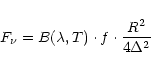
For the comets, we determined 36 "hits'' where the object was within
5![]() from the slew centre and with the comet being within 3 AU
(for Hale-Bopp 5 AU) from the Sun. A simple flux estimate lowered
the number to 16 possible candidates. The 170
from the slew centre and with the comet being within 3 AU
(for Hale-Bopp 5 AU) from the Sun. A simple flux estimate lowered
the number to 16 possible candidates. The 170 ![]() m
flux estimate was based on an assumed dust albedo A=0.10 and a temperature
of dust particles of T0=330 K at the heliocentric distance of r=1 AU
through the following formula:
m
flux estimate was based on an assumed dust albedo A=0.10 and a temperature
of dust particles of T0=330 K at the heliocentric distance of r=1 AU
through the following formula:
 |
(1) |
The search radius for each pointing had to be much bigger than the
real
![]() field of view of the detector
for several reasons: 1) slew position uncertainties (up to 2
field of view of the detector
for several reasons: 1) slew position uncertainties (up to 2![]() ,
Stickel et al. 2000);
2) uncertainties of the 2-body unperturbed ephemeris, based on 200-day
epoch orbital elements (up to a few arcmin); 3) the ISO parallax
(up to 3
,
Stickel et al. 2000);
2) uncertainties of the 2-body unperturbed ephemeris, based on 200-day
epoch orbital elements (up to a few arcmin); 3) the ISO parallax
(up to 3![]() for close encounters at 0.5 AU).
In the first iteration, the search radii were set to 8.1
for close encounters at 0.5 AU).
In the first iteration, the search radii were set to 8.1![]() for
asteroids (3
for
asteroids (3![]() for ephemeris uncertainties, 3
for ephemeris uncertainties, 3![]() for
ISO parallax, 2.1
for
ISO parallax, 2.1![]() for the centre-corner distance of
the C200 array), to 30
for the centre-corner distance of
the C200 array), to 30![]() for comets (to account for extended
structures) and to 2
for comets (to account for extended
structures) and to 2![]() for the bright planets (to account for
possible straylight influences). In the second iteration, after the
ephemeris recalculation with an N-body programme and after parallax
corrections, the search radius was uniformly set to 5
for the bright planets (to account for
possible straylight influences). In the second iteration, after the
ephemeris recalculation with an N-body programme and after parallax
corrections, the search radius was uniformly set to 5![]() .
Additionally, all identified slews from the first iteration were
marked, because of possible influences from bright SSOs.
.
Additionally, all identified slews from the first iteration were
marked, because of possible influences from bright SSOs.
Figure 3 summarizes the procedure in detail,
giving also the input and output number of targets.
With this procedure it was possible to reduce the initially estimated
1011 ephemeris calculations to 109 2-body and 104 N-body calculations.
The final potential hits of 56 asteroids, 16 comets and 22 planets
fulfilled the flux requirements at the actual time of the observation
and were located within 5![]() of the slew.
Note that we count each encounter of a slew with an SSO as
"hit''. The actual numbers of different objects in this list are
21 asteroids, 7 comets and 2 planets.
These results, based on pure pointing and timing information, are strongly
influenced and biased by the unequal distribution of the slews in the sky,
satellite visibility constraints and the ISO observing programme itself.
The relatively large number of comets is
due to the weak flux limit and it was clear that not all of them would be
bright enough to be detected.
of the slew.
Note that we count each encounter of a slew with an SSO as
"hit''. The actual numbers of different objects in this list are
21 asteroids, 7 comets and 2 planets.
These results, based on pure pointing and timing information, are strongly
influenced and biased by the unequal distribution of the slews in the sky,
satellite visibility constraints and the ISO observing programme itself.
The relatively large number of comets is
due to the weak flux limit and it was clear that not all of them would be
bright enough to be detected.
ISOSS observations of Uranus, Neptune and well known bright asteroids enabled us to improve and extend the existing ISOSS calibration (Method 1). They also allowed us to estabish the calibration of new source and flux extraction methods, namely Methods 2, 3a and 3b (see Sect. 2).
The Uranus and Neptune models are based on Griffin & Orton (1993) and Orton & Burgdorf (priv. comm.), respectively. For Ceres, Pallas, Juno and Vesta a thermophysical model (TPM) (Lagerros 1996, 1997, 1998) was used to predict their brightnesses at the times of the observations. The TPM and its input parameters are described in Müller & Lagerros (1998) and in Müller et al. (1999). The quality and final accuracy of TPM predictions are discussed in Müller & Lagerros (2002a). The general aspects of asteroids as calibration standards for IR projects are summarized in Müller & Lagerros (2002b).
Photometric measurements of different astronomical sources can
be compared on the basis of colour corrected monochromatic fluxes
at a certain wavelength or on the basis of band pass fluxes.
In this calibration section all model fluxes have been modified by an
"inverse colour correction''
in a way that they correspond to ISOSS band pass measurements
of a constant energy spectrum (
![]() ). This
implied inverse colour correction terms of 1.09-1 for Uranus
and Neptune (both have temperatures at around 60 K at 170
). This
implied inverse colour correction terms of 1.09-1 for Uranus
and Neptune (both have temperatures at around 60 K at 170 ![]() m)
and 1.17-1 for the bright main-belt asteroids (assumed far-IR
temperature of 180-200 K), see also the colour correction tables
in "The ISO Handbook, Volume V'', Laureijs et al. (2000).
m)
and 1.17-1 for the bright main-belt asteroids (assumed far-IR
temperature of 180-200 K), see also the colour correction tables
in "The ISO Handbook, Volume V'', Laureijs et al. (2000).
| TDT | Date/Time | SSO |
|
|
|
| No. | (Jy) | (Jy) | |||
| (1) | (2) | (3) | (4) | (5) | (6) |
| 07881200 | 03-Feb.-96 09:46:42 | (4) Vesta | 28.9 | 39.6 | 0.73 |
| 10180400 | 26-Feb.-96 06:20:00 | (4) Vesta | 30.7 | 54.2 | 0.57 |
| 14080700 | 05-Apr.-96 15:39:10 | Neptune | 145.1 | 271.3 | 0.53 |
| 23080100 | 03-Jul.-96 20:15:13 | (2) Pallas | 15.2 | 27.5 | 0.55 |
| 32181100 | 03-Oct.-96 04:38:13 | Neptune | 153.2 | 279.8 | 0.55 |
| 42283300 | 11-Jan.-97 22:47:14 | (3) Juno | 12.6 | 12.0 | 1.05 |
| 34480700 | 26-Oct.-96 00:25:16 | Neptune | 159.1 | 272.7 | 0.58 |
| 69880600 | 13-Oct.-97 21:27:19 | Neptune | 160.7 | 277.6 | 0.58 |
| 70681100 | 22-Oct.-97 02:44:35 | Neptune | 158.0 | 274.9 | 0.57 |
| 71381000 | 29-Oct.-97 05:06:45 | Neptune | 168.3 | 272.7 | 0.62 |
| 71980500 | 03-Nov.-97 22:46:18 | Neptune | 149.9 | 271.3 | 0.55 |
| 72081500 | 05-Nov.-97 01:19:05 | Uranus | 395.7 | 672.8 | 0.59 |
| 72081600 | 05-Nov.-97 01:57:38 | Neptune | 156.1 | 270.5 | 0.58 |
| 76280400 | 16-Dec.-97 13:22:05 | (1) Ceres | 31.5 | 52.4 | 0.60 |
| 79781500 | 21-Jan.-98 00:30:12 | (4) Vesta | 24.2 | 23.9 | 1.01 |
ISOSS crossings over planets and asteroids, which were detected by the
Automatic Point Source Extractor (Stickel et al. 2000),
are listed in Table 1,
where the columns are: (1) TDT number of
the slew, (2) date and Universal Time at the moment of the SSO
observation, (3) name of the solar system object,
(4) observed flux density, (5) predicted flux density, (6)
ratio between observed and modeled flux density (see also
Fig. 4). The ISOSS results are
the FCS calibrated band fluxes. The model predictions were modified
by an inverse colour correction to make them comparable with the
ISOSS measurements (see above).
All list entries of Uranus, Neptune, Ceres, Pallas and Vesta give a ratio
between observed and model flux of (0.58 ![]() 0.05), for fluxes
larger than about 25 Jy. At fluxes below 25 Jy (only 2 cases) the
ISOSS to model ratios are close to 1.0.
This is in excellent agreement with the results of Stickel et al. (2000).
They showed that ISOSS slew fluxes of 12 selected galaxies were
systematically lower than fluxes derived from dedicated maps. To
bring the fluxes from mapping and slewing into agreement
ISOSS fluxes larger than
0.05), for fluxes
larger than about 25 Jy. At fluxes below 25 Jy (only 2 cases) the
ISOSS to model ratios are close to 1.0.
This is in excellent agreement with the results of Stickel et al. (2000).
They showed that ISOSS slew fluxes of 12 selected galaxies were
systematically lower than fluxes derived from dedicated maps. To
bring the fluxes from mapping and slewing into agreement
ISOSS fluxes larger than ![]() 30 Jy were corrected with an
estimated constant scaling factor of 2, while lower fluxes were scaled
with a flux dependent correction function.
Table 1 represents therefore the first direct flux
calibration of the PHT Serendipity Mode as compared to the previously
used indirect method of flux ratios between PHT22 raster maps and slew
results.
30 Jy were corrected with an
estimated constant scaling factor of 2, while lower fluxes were scaled
with a flux dependent correction function.
Table 1 represents therefore the first direct flux
calibration of the PHT Serendipity Mode as compared to the previously
used indirect method of flux ratios between PHT22 raster maps and slew
results.
![\begin{figure}
\par\includegraphics[angle=90,width=8.8cm,clip]{tmueller_fig4.ps}
\end{figure}](/articles/aa/full/2002/26/aa2270/img34.gif) |
Figure 4: The ratio of Serendipity slew flux densities and model predictions for reliable Uranus, Neptune, Ceres, Pallas, Juno and Vesta observations. For bright sources, the Serendipity slews miss some flux. |
| Open with DEXTER | |
Figure 4 shows the ratios
between the flux densities derived from ISOSS and the 170 ![]() m
model predictions. The stars represent the results from dedicated
calibration measurements (Stickel et al. 2000), the
filled circles are values from Table 1.
Uranus, Neptune, Ceres, Pallas, Juno and Vesta, serendipitously seen
by ISOSS, provide now a reliable calibration at higher flux densities.
m
model predictions. The stars represent the results from dedicated
calibration measurements (Stickel et al. 2000), the
filled circles are values from Table 1.
Uranus, Neptune, Ceres, Pallas, Juno and Vesta, serendipitously seen
by ISOSS, provide now a reliable calibration at higher flux densities.
Table 2 summarizes the values which were derived from the solar system far-IR standards for slow slewing speeds, saturated measurements and sources outside the slews. These measurements were rejected by the source extraction procedures of Method 1. The table columns are: (1-6) same as in Table 1, (7) slew speed category at the moment of the SSO observation, (8) additional remarks.
| TDT | Date/Time | SSO |
|
|
|
Slew speed | Remarks |
| No. | (Jy) | (Jy) | |||||
| (1) | (2) | (3) | (4) | (5) | (6) | (7) | (8) |
| 09380600 | 18-Feb.-96 15:10:15 | (1) Ceres | >46 | 73.8 | >0.62 | slow | ok |
| 29280600 | 04-Sep.-96 00:31:59 | (1) Ceres | >54 | 67.2 | >0.80 | slow | very high bgd. |
| 32880600 | 09-Oct.-96 23:11:09 | Neptune | >155 | 277.8 | >0.56 | slow | ok |
| 36381700 | 14-Nov.-96 04:34:23 | Neptune | 267.2 | moderate | outside | ||
| 54480800 | 13-May.-97 12:58:55 | Uranus | 700.1 | moderate | saturated | ||
| 55280300 | 21-May.-97 06:17:09 | Uranus | 709.5 | stop | outside | ||
| 69880200 | 13-Oct.-97 17:39:49 | Uranus | 700.1 | moderate | saturated | ||
| 69880500 | 13-Oct.-97 20:48:47 | Uranus | 700.1 | moderate | saturated | ||
| 71480300 | 29-Oct.-97 23:34:32 | Uranus | 680.8 | moderate | saturated | ||
| 87481000 | 07-Apr.-98 14:36:41 | Uranus | 652.0 | moderate | saturated |
The results from Method 2 show that also difficult slew data with either saturated pixels, objects slightly outside the array or slow speeds can be used to derive useful lower limits for interesting sources. As the satellite still moves the flux loss corrections from Method 1 have to be applied to get the best lower limits. In fact, for the 2 unproblematic hits (TDT 9380600 and 32880600) with neither saturated signals nor large impact parameters, the flux loss correction brings the ISOSS fluxes within 10% of the model predictions.
At the slewend, when the satellite does not move anymore, the ISOSS data can in principle be treated as normal C200 photometric data. Two ideal cases - source centred on the array (Method 3a) and source centred on one pixel (Method 3b) - can be distinguished. The results on the bright sources for both methods are summarized in Table 3, where the columns are the same as in Table 1. The uncertainties in the table, given in brackets, are statistical errors of weighted results from all 4 pixels. The results of Method 3 are compared with the model predictions in Fig. 5.
![\begin{figure}
\par\includegraphics[width=8.8cm,clip]{tmueller_fig5.ps}
\end{figure}](/articles/aa/full/2002/26/aa2270/img35.gif) |
Figure 5: The ratio of Serendipity flux densities from Method 3a and model predictions for Neptune, Ceres, Pallas, Juno and Vesta observations. Error bars are statistical errors from the individual pixel results. Circles encompass data points from slews which had to be calibrated with the default calibration; in these cases, the true uncertainties exceed the given statistical errors. A flux dependency similar as in Fig. 4 (Method 1) can be seen. |
| Open with DEXTER | |
| TDT | Date/Time | SSO |
|
|
|
| No. | (Jy) | (Jy) | |||
| (1) | (2) | (3) | (4) | (5) | (6) |
| 09380500 | 18-Feb.-96 07:11:04 | (1) Ceres | 70.1(6.9) | 74.4 | 0.94 |
| 15480200 | 19-Apr.-96 03:42:10 | Neptune | 269(11.1) | 275.3 | 0.98 |
| 23781000 | 11-Jul.-96 04:13:16 | (3) Juno | 12.9(2.6) | 9.5 | 1.35 |
| 25180400 | 24-Jul.-96 23:47:09 | (2) Pallas | 26.4(2.0) | 22.3 | 1.18 |
| 26580800 | 08-Aug.-96 02:50:48 | (2) Pallas | 25.1(2.4) | 19.5 | 1.29 |
| 27580200 | 18-Aug.-96 02:17:46 | (1) Ceres | 85.2(10.2) | 79.4 | 1.07 |
| 32880500 | 09-Oct.-96 21:54:26 | Neptune | 236(18.3) | 277.8 | 0.85 |
| 35680200 | 06-Nov.-96 20:07:37 | Neptune | 267(16.1) | 269.3 | 0.99 |
| 38781200 | 07-Dec.-96 23:52:44 | (3) Juno | 22.4(5.4) | 15.6 | 1.44 |
| 41980900 | 08-Jan.-97 18:53:29 | (3) Juno | 16.3(0.5) | 12.5 | 1.30 |
| 51080600 | 09-Apr.-97 10:54:42 | (2) Pallas | 14.1(2.1) | 10.8 | 1.30 |
| 51080800 | 09-Apr.-97 15:19:52 | (2) Pallas | 16.1(1.3) | 10.5 | 1.53 |
| 51380100 | 12-Apr.-97 04:33:19 | (2) Pallas | 16.7(3.9) | 11.5 | 1.45 |
| 53980100 | 08-May-97 03:39:36 | Neptune | 282(70.4) | 280.8 | 1.00 |
| 53980300 | 08-May-97 11:11:10 | Neptune | 278(31.1) | 280.8 | 0.99 |
| 54581400 | 14-May-97 10:49:26 | (1) Ceres | 67.2(4.3) | 55.5 | 1.21 |
| 57581500 | 13-Jun.-97 13:53:04 | (4) Vesta | 32.5(2.9) | 24.6 | 1.32 |
| 74881000 | 03-Dec.-97 02:21:54 | (1) Ceres | 67.1(3.5) | 58.3 | 1.15 |
| 53880300 | 07-May-97 07:54:19 | (1) Ceres | 43.8(4.9) | 52.5 | 0.83 |
| 61580800 | 23-Jul.-97 02:07:07 | (4) Vesta | 31.1(1.2) | 34.4 | 0.91 |
The 5 Neptune measurements (Method 3a) agree nicely with the
model predictions (Observation/Model: 0.96 ![]() 0.09).
For the fainter asteroids the Method 3a overestimates the flux
systematically by 10-50%, depending on the brightness level
(see Fig. 5).
The discrepancy between bright and faint sources is probably due to
detector nonlinearities,
which are not corrected in the OLP 7 Serendipity Mode
data, and which could be responsible for the flux dependency of the
scaling factor (see Sect. 4.1).
A comparison of Fig. 5 with Fig. 4 supports this
explanation, as both diagrams show a decrease in the detector
signals for bright sources. The fast slewing on the other hand,
which affects Method 1 but not Method 3, could be responsible for
the generally too low ISOSS fluxes in Fig. 4.
0.09).
For the fainter asteroids the Method 3a overestimates the flux
systematically by 10-50%, depending on the brightness level
(see Fig. 5).
The discrepancy between bright and faint sources is probably due to
detector nonlinearities,
which are not corrected in the OLP 7 Serendipity Mode
data, and which could be responsible for the flux dependency of the
scaling factor (see Sect. 4.1).
A comparison of Fig. 5 with Fig. 4 supports this
explanation, as both diagrams show a decrease in the detector
signals for bright sources. The fast slewing on the other hand,
which affects Method 1 but not Method 3, could be responsible for
the generally too low ISOSS fluxes in Fig. 4.
Both options of Methods 3 open a powerful new possibility to
evaluate the 170 ![]() m fluxes of many scientific ISO targets,
which are quite often covered in the end of slews before the
intended science programme starts.
m fluxes of many scientific ISO targets,
which are quite often covered in the end of slews before the
intended science programme starts.
The N-body ephemeris calculations for our SSOs included
a transformation from geocentric to ISOcentric frame.
The maximal geo-/ISOcentric parallax corrections
were: 737.7
![]() for the Apollo asteroid (7822) 1991 CS,
336.6
for the Apollo asteroid (7822) 1991 CS,
336.6
![]() comet P/Encke and 61.2
comet P/Encke and 61.2
![]() for
Mars. The final accuracy of the ISOcentric SSO ephemeris has been
estimated to about 1-2
for
Mars. The final accuracy of the ISOcentric SSO ephemeris has been
estimated to about 1-2
![]() .
.
The ISOSS signal pattern, i.e. the relative signals of the 4 pixels,
is a very sensitive indicator of the exact position of
the source within the detector array.
All close encounters have been checked by eye for
discrepancies between predicted slew offsets and the signal patterns.
No disagreement was found, which implies that the predicted SSO positions
and the slew positions agree with each other within 30
![]() ,
corresponding to 1/3 pixel width. In case of non-detections, the SSOs
were either too faint, or they were actually just
outside the slew. This high pointing accuracy allowed
us to give upper limits (depending on the background) in cases
when the source was crossed by the slew but no signal was
detected (see also Sect. 2.2.2).
In slew direction the position accuracy is better
than 1
,
corresponding to 1/3 pixel width. In case of non-detections, the SSOs
were either too faint, or they were actually just
outside the slew. This high pointing accuracy allowed
us to give upper limits (depending on the background) in cases
when the source was crossed by the slew but no signal was
detected (see also Sect. 2.2.2).
In slew direction the position accuracy is better
than 1![]() ,
limited by fast slewing in combination with
the detector read-out frequency.
,
limited by fast slewing in combination with
the detector read-out frequency.
The procedure from Sect. 3 resulted in a list of potential SSO candidates in the ISOSS. Mainly for the following reasons, not all of them were visible in the slew data:
In some cases the object was visible, but a reliable flux determination from the ISOSS was not possible. In these cases upper or lower limits are given.
Tables 4, 5 and 6
include all SSO predictions which are within 5![]() of
the slew centre, fulfill the flux requirements and have not been used
in Sect. 4.
For the scientific comparison between ISOSS fluxes and model predictions
we did the following calibration steps: We determined the ISOSS calibrated
inband fluxes through the
different methods and corrected them by an
estimated factor based on the slopes visible in Figs. 4
and 5. As a last step we applied the colour correction to
obtain monochromatic flux densities at 170
of
the slew centre, fulfill the flux requirements and have not been used
in Sect. 4.
For the scientific comparison between ISOSS fluxes and model predictions
we did the following calibration steps: We determined the ISOSS calibrated
inband fluxes through the
different methods and corrected them by an
estimated factor based on the slopes visible in Figs. 4
and 5. As a last step we applied the colour correction to
obtain monochromatic flux densities at 170 ![]() m
(ISOSS values in Tables 4, 5).
m
(ISOSS values in Tables 4, 5).
The inner planets were not visible for ISO due to pointing
constraints. Mars, Jupiter and Saturn exceeded the saturation
limits, Pluto was below the 1.0 Jy limit. Therefore, only
Uranus and Neptune were seen, but were already used to extend the ISOSS
calibration (Sects. 4.1, 4.2
and 4.3). However, the bright planets had to be included
in the search programme with the objective to identify close-by slews.
For the extremely IR bright planets, diffraction effects of the optical
system in combination with certain satellite-planet constellations produced
bright spots, spikes and ring like structures around the planets,
which are visible in the slew data. Mars, Jupiter and Saturn, with
170 ![]() m brightnesses between 10 000 and 400 000 Jy, influenced
slews up to 1
m brightnesses between 10 000 and 400 000 Jy, influenced
slews up to 1![]() distance, Uranus and Neptune (>200 Jy)
up to 10
distance, Uranus and Neptune (>200 Jy)
up to 10![]() distance. These slews have been identified
(with the above mentioned SSO extraction method in combination with a large
search radius) and the planet influence can now be taken into
account for further scientific catalogues based on ISOSS.
Some planetary satellites are bright enough to be visible in principle.
However, close to Jupiter (the maximal distance for the Galilean
satellites is about 11
distance. These slews have been identified
(with the above mentioned SSO extraction method in combination with a large
search radius) and the planet influence can now be taken into
account for further scientific catalogues based on ISOSS.
Some planetary satellites are bright enough to be visible in principle.
However, close to Jupiter (the maximal distance for the Galilean
satellites is about 11![]() )
and Saturn (the maximal angular
distance for the 8 largest satellites is about 10
)
and Saturn (the maximal angular
distance for the 8 largest satellites is about 10![]() )
no
170
)
no
170 ![]() m fluxes can be derived, due to the strong planet influences.
m fluxes can be derived, due to the strong planet influences.
The measured Uranus and Neptune flux values from
Tables 1, 2 and 3
can also be used as input to future models of planetary atmospheres.
Current models are based on Voyager IRIS data from 25 to 50 ![]() m
and sub-millimetre data beyond 350
m
and sub-millimetre data beyond 350 ![]() m (Griffin & Orton
1993) with an interpolation in between. The ISOSS
observations make this wavelength range directly accessible for
model tests in the far-IR.
m (Griffin & Orton
1993) with an interpolation in between. The ISOSS
observations make this wavelength range directly accessible for
model tests in the far-IR.
After establishing new methods for the flux calibration, based now
additionally on measurements of Uranus, Neptune,
Ceres, Pallas, Juno and Vesta,
the monochromatic flux densities at 170 ![]() m of the remaining
asteroids were derived. 23 out of the 56 asteroid "hits''
were already used in this calibration context in the previous
Sect. 4. The remaining 33 hits can be split in 3 groups:
m of the remaining
asteroids were derived. 23 out of the 56 asteroid "hits''
were already used in this calibration context in the previous
Sect. 4. The remaining 33 hits can be split in 3 groups:
18 asteroid predictions have reliable IRAS detections, but only low quality ISOSS detections. The reasons for the poor ISOSS fluxes are manifold: slew offsets, bright backgrounds, technical problems, low fluxes, etc. For these 18 asteroids Tedesco et al. (1992) calculated already diameters and albedos, based on IRAS observations. Upper flux limits from ISOSS would therefore not give any new information.
| TDT | Date/Time | SSO |
|
|
Method | Slew | Remarks |
| No. | (Jy) | (Jy) | speed | ||||
| (1) | (2) | (3) | (4) | (5) | (6) | (7) | (8) |
| 11080300 | 06-Mar.-96 11:42:00 | (5) Astraea | <4 | 1.3 | 2 | fast | upper limit, cirrus bgd. |
| 12780300 | 23-Mar.-96 02:50:17 | (5) Astraea | <4 | 1.6 | 2 | fast | upper limit, cirrus bgd. |
| 85480200 | 18-Mar.-98 13:48:12 | (7) Iris | <3 | 2.1 | 2 | fast | in cirrus knot |
| 25381400 | 27-Jul.-96 03:22:14 | (15) Eunomia | 2.9 | 2.5 | 1 | fast | ok |
| 85480300 | 18-Mar.-98 17:22:43 | (89) Julia | <3 | 1.7 | 2 | fast | upper limit |
| 18780100 | 22-May-96 05:40:00 | (344) Desiderata | 4.5 | 5.8 | 1 | fast | ok |
| 18280800 | 17-May-96 03:50:00 | (532) Herculina | 5.3(1.0) | 5.5 | 3a | stop | ok |
| 21780900 | 21-Jun.-96 06:01:48 | (532) Herculina | 3.4(0.3) | 3.8 | 3a | stop | ok |
| 83380500 | 25-Feb.-98 11:36:26 | (1036) Ganymed | <4 | 0.1 | 2 | fast | upper limit |
7 asteroids (9 hits) have reliable IRAS detections and also good quality ISOSS detections (see Table 4). For these asteroids we could successfully derive fluxes and upper limits with our newly established calibration, based on clear detections. The IRAS diameter and albedo values in the following are all taken from the Minor Planet Survey (MPS, Tedesco et al. 1992).
| TDT | Date/Time | SSO |
|
|
Method | Slew | Real source | Remarks |
| No. | (Jy) | (Jy) | speed | offset |
||||
| (1) | (2) | (3) | (4) | (5) | (6) | (7) | (8) | (9) |
| 83081700 | 22-Feb.-98 19:07:18 | (9) Metis | 3.8 | 4.1 | 1 | fast | 0 |
ok |
| 84281000 | 06-Mar.-98 16:31:55 | (9) Metis | >1 | 3.4 | 2 | fast | 0.3 |
|
| 63681300 | 13-Aug.-97 10:42:38 | (27) Euterpe | -- | 1.5 | -- | fast | 1.9 |
no detection |
| 25880900 | 01-Aug.-96 07:42:48 | (391) Ingeborg | -- | 0.2 | -- | fast | 2.5 |
no detection |
| 71682300 | 01-Nov.-97 06:03:56 | (3753) Cruithne | -- | 0.1 | -- | fast | 1.0 |
no detection |
| 27482100 | 17-Aug.-96 01:22:01 | (7822) 1991 CS | -- | 0.1 | -- | fast | 2.5 |
no detection |
5 asteroids (6 hits) have no IRAS detection, but fulfilled the conservative flux requirements for the ISOSS asteroid search (see Table 5). Unfortunately 4 sources (Euterpe, Ingeborg, Cruithne and 1991 CS) have only marginal ISOSS detections and establishing upper flux limits was difficult. The results of Table 5 per Object:
Based on the ISOSS flux of 3.8 Jy, the TPM allowed the calculation
of an effective projected diameter of 178 km and an albedo
of pV=0.15 at the epoch of the ISOSS observation.
A possible 20% ISOSS flux uncertainty would correspond to
about 10% diameter uncertainty, resulting in a
size of the rotating ellipsoid of
![]() km with 10% minimum uncertainties.
km with 10% minimum uncertainties.
Within the different uncertainties and based on the shape and spin vector solutions, the results agree nicely. The 3 methods - occultation, HST direct imaging and ISOSS radiometric method - led to comparable diameters and albedos.
The Juno observations in Tables 1 and 3 have flux ratios systematically higher than
ratios from comparable sources.
Calibrating the ISOSS values with the corresponding newly established
methods 1 and 3a resulted in an average observation over model ratio
of 1.14, indicating that the model diameter of Juno is about
7% too low. Müller & Lagerros (2002a) analysed 11
independent ISO observations, taken with the long wavelengths ISOPHOT
detectors. They find a similar mean ratio of 1.13 ![]() 0.10, which
confirms the tendency to higher diameter values. Both investigations
indicate that the effective diameter should be close to 260 km, compared
to the published values of 241.4 km (Müller & Lagerros 1998)
and 233.9
0.10, which
confirms the tendency to higher diameter values. Both investigations
indicate that the effective diameter should be close to 260 km, compared
to the published values of 241.4 km (Müller & Lagerros 1998)
and 233.9 ![]() 11.2 km (Tedesco et al. 1992).
11.2 km (Tedesco et al. 1992).
For Vesta the situation is not that clear. The values in Table 1 are not conclusive since the Vesta fluxes cover the difficult transition region between little flux loss and the more than 40% flux loss for sources brighter than 25 Jy (see Fig. 4). It seems that two of the measured fluxes (TDT 07881200, 79781500) are higher than one would expect from other sources with similar brightness. This contradicts the findings by Redman et al. (1998; 1992). They state for Vesta an extremely low emissivity of 0.6 in the submillimetre. Assuming that the emissivity is already lower in the far-IR would mean that the Vesta points in Fig. 4 should lie below the general trend and not above. The measurement from methods 3a (TDT 57581500) and 3b (TDT 61580800) agree within the errorbars with the model predictions. As in Müller & Lagerros (2002a), we see no clear indications of far-IR emissivities lower than the default values given in Müller & Lagerros (1998)
| TDT | Date/Time | SSO | RA | Dec. | r |
|
|
|
| No. | (hms) | (dms) | (AU) | (AU) | (Jy) | (Jy) | ||
| (1) | (2) | (3) | (4) | (5) | (6) | (7) | (8) | (9) |
| 60780100 | 14-Jul.-97 22:57:49 | 2P/Encke | 14 56 28.6 | -63 36 09 | 1.164 | 0.264 | 5-10 | >50 |
| 34881300 | 29-Oct.-96 22:27:01 | 22P/Kopff | 21 23 56.6 | -19 53 22 | 1.961 | 1.523 | 0.5-1 | <1 |
| 23380800 | 07-Jul.-96 11:31:51 | 96P/Machholz 1 | 23 10 27.5 | -68 19 46 | 2.052 | 1.328 | no det. | |
| 77780200 | 31-Dec.-97 16:38:09 | 103P/Hartley 2 | 23 27 54.1 | -07 29 09 | 1.041 | 0.825 | poor det. | |
| 80280100 | 25-Jan.-98 15:07:48 | 104P/Kowal 2 | 00 43 46.0 | +08 38 35 | 1.451 | 1.496 | 1 | |
| 33280100 | 13-Oct.-96 18:43:22 | 126P/IRAS | 21 38 46.7 | -29 54 48 | 1.712 | 1.028 | -- | >2 |
| 36280400 | 12-Nov.-96 13:51:16 | 126P/IRAS | 21 45 50.3 | -08 47 05 | 1.709 | 1.307 | 1.0 | <2 |
| 13481800 | 30-Mar.-96 17:26:33 | C/1995 O1 = | 19 42 20.5 | -19 43 10 | 4.867 | 5.004 | see text | |
| 16280600 | 27-Apr.-96 14:17:19 | Hale-Bopp | 19 44 35.1 | -17 37 42 | 4.588 | 4.259 | 9.3 |
|
| 31580500 | 27-Sep.-96 0:05:16 |
|
17 29 43.0 | -05 11 32 | 2.934 | 2.965 | 30.9 |
|
| 32081300 | 01-Oct.-96 17:21:44 |
|
17 29 42.8 | -04 57 58 | 2.878 | 2.987 | see text | |
| 32280200 | 03-Oct.-96 15:16:59 |
|
17 29 50.7 | -04 52 28 | 2.856 | 2.995 | see text | |
| 32580600 | 06-Oct.-96 23:28:20 |
|
17 30 13.8 | -04 42 47 | 2.816 | 3.009 | see text | |
| 77081500 | 25-Dec.-97 0:18:51 |
|
06 32 55.7 | -64 09 08 | 3.851 | 3.683 | 43.8 |
|
| 86880300 | 01-Apr.-98 14:02:15 |
|
05 02 13.8 | -53 09 12 | 4.855 | 4.945 | see text | |
| 87380400 | 06-Apr.-98 16:12:29 |
|
05 05 07.0 | -52 34 21 | 4.905 | 5.009 | 15.0 |
![\begin{figure}
\par\includegraphics[width=8.8cm,clip]{tmueller_fig6.ps}
\end{figure}](/articles/aa/full/2002/26/aa2270/img56.gif) |
Figure 6:
An ISOSS profile of Hale-Bopp in comparison
with the signal pattern of a point source. The slewing
speeds for these two hits were identical and already quite low
(2 |
| Open with DEXTER | |
The fluxes derived from Method 3a can be compared to results from
Grün et al. 2001 through the following corrections:
1) Flux corrections according to Fig. 5;
2) Normalization to a standard aperture diameter of 23![]() assuming that the coma brightness scales linearly with
aperture diameter (
ca23=0.120);
3) Point-spread-function correction which takes into account
the differences of a point source and a
assuming that the coma brightness scales linearly with
aperture diameter (
ca23=0.120);
3) Point-spread-function correction which takes into account
the differences of a point source and a ![]() -coma
(
-coma
(
![]() );
4) Colour correction
);
4) Colour correction![]() which changes for different distances
from the sun (
which changes for different distances
from the sun (
![]() ).
).
The first two measurements (16280600, 31580500) were obtained
on the same days as the ones in Grün et al. (2001).
The calibrated and reduced 23![]() fluxes agree within
the errorbars. The third observation (77081500), taken 5 days
earlier than the dedicated Hale-Bopp observation,
lead to a flux of 5.64
fluxes agree within
the errorbars. The third observation (77081500), taken 5 days
earlier than the dedicated Hale-Bopp observation,
lead to a flux of 5.64 ![]() 0.56 Jy, as compared to 2.66 Jy.
This large difference can not be explained by epoch or geometry
differences. However, the dedicated measurement was mis-pointed
by 24
0.56 Jy, as compared to 2.66 Jy.
This large difference can not be explained by epoch or geometry
differences. However, the dedicated measurement was mis-pointed
by 24![]() which caused large uncertainties in the applied
corrections. The ISOSS flux provides therefore valuable information
for the colour temperature determination and, through grain size
models, might give clues whether icy grains were present in the coma
in December 1997 at almost 4 AU post-perihelion.
The last measurement of Method 3a (87380400) was obtained when
Hale-Bopp was already 4.9 AU from the sun. The
calibrated and reduced 23
which caused large uncertainties in the applied
corrections. The ISOSS flux provides therefore valuable information
for the colour temperature determination and, through grain size
models, might give clues whether icy grains were present in the coma
in December 1997 at almost 4 AU post-perihelion.
The last measurement of Method 3a (87380400) was obtained when
Hale-Bopp was already 4.9 AU from the sun. The
calibrated and reduced 23![]() flux was 1.97
flux was 1.97 ![]() 0.39 Jy.
This is the most distant thermal far-IR observation of Hale-Bopp
post-perihelion. A comparison of the flux with a dedicated
observation (Grün et al. 2001;
0.39 Jy.
This is the most distant thermal far-IR observation of Hale-Bopp
post-perihelion. A comparison of the flux with a dedicated
observation (Grün et al. 2001;
![]() Jy) at
a similar distance from the sun, but pre-perihelion, shows that the
dust emission post-perihelion was higher as the comet receeded from
the sun. In fact, the higher far-IR fluxes post-perihelion are
related to contributions from large particles which have been
accumulated during the passage around the sun and which stay on
similar orbits as the nucleus.
Jy) at
a similar distance from the sun, but pre-perihelion, shows that the
dust emission post-perihelion was higher as the comet receeded from
the sun. In fact, the higher far-IR fluxes post-perihelion are
related to contributions from large particles which have been
accumulated during the passage around the sun and which stay on
similar orbits as the nucleus.
Two measurements (32280200, 86880300) show signal peaks a few arcminutes away from the nucleus in anti-orbital velocity (trail) direction. It seems that the emitting dust particles are not homogeneously distributed and are concentrated in a narrow region of the outer parts of the dust coma towards the trail direction. These features are not seen in slews over other parts of the outer coma. Reach et al. (2000) observed for the first time the dust trail formation in comet Encke in the mid-IR. The ISOSS data provide now evidence for this process in the far-IR where the emission is strongly connected to the largest particles.
The purpose of the SSO extraction from the ISOSS was manifold: Calibration aspects, catalogue cleaning aspects and scientific aspects. The main achievements were clearly in the calibration section, were serendipitously seen asteroids and planets led to an improved flux calibration for ISOSS targets. Bright sources of the automatic point-source extraction procedure have now a solid calibration basis. It was also possible to establish new methods to calibrate source detections under a large variety of circumstances, including the important slew end positions and low slewing speeds.
The aspect of SSO cleaning from ISOSS catalogue lists will avoid wrong identifications and help follow up programmes of galactic and extra-galactic sources.
The outcome of the scientific analysis of SSO detections were modest
due to the limitations of the ISOSS mentioned in Sect. 5.
Despite all difficulties we could demonstrate that the far-IR fluxes
of asteroids are important. Diameter and albedo estimates through
TPM calculations are much more reliable than estimates based on
visible brightness alone. An accurate H-value of 12.0 mag would
allow for diameters ranging from 10.6 km (pV=0.25) to 23.7 km
(pV=0.05), corresponding to a ![]() 40% uncertainty of the
average. An additional thermal flux with a flux error of
40% uncertainty of the
average. An additional thermal flux with a flux error of ![]() 20%
allows a 4 times more accurate diameter determination.
20%
allows a 4 times more accurate diameter determination.
The ISOSS results for Hale-Bopp are more valuable. They can now be used for additional comet modeling (e.g. models by Hanner 1983) for more reliable interpretation of grain properties and ice influences at different heliocentric distances. Comets are usually optically bright due to fresh ice surfaces, but in the far-IR the sublimated larger particles dominate the thermal emission. After many orbits around the sun these large particles form trails which were first measured by IRAS (Sykes 1986). For Hale-Bopp we found significantly more thermal emission post-perihelion than for comparable configurations pre-perihelion. Additionally we saw asymmetries due to the dust tail and an indicative detection of large particles concentrated towards the anti-orbital velocity (trail) direction.
The expectations for future far-IR and submillimetre projects on
SSO related topics are large: SIRTF, SOFIA, ASTRO-F, HERSCHEL
and others will have many dedicated programmes on asteroids,
comets and planets, but will also see by chance interesting targets.
Especially the ASTRO-F/FIS all sky survey in 4 photometric bands
in the region 50 to 200 ![]() m will serendipitously detect
many SSOs. Our experience with ISOSS in terms of calibration
through asteroids and planets, but also in identification of
moving targets could then be of great benefit.
m will serendipitously detect
many SSOs. Our experience with ISOSS in terms of calibration
through asteroids and planets, but also in identification of
moving targets could then be of great benefit.
Acknowledgements
We would like to thank Elwood C. Downey for many helpful discussions and for providing xephemdbd for position calculation of SSOs.The orbital elements were provided by Gareth Williams, IAU Minor Planet Center (http://cfa-www.harvard.edu/~iau/mpc.html), for 4 epochs during the ISO mission: 1996 Apr. 27, 1996 Nov. 13, 1997 Jun. 1 and 1997 Dec. 18. A modified version of the Uppsala N-body ephemeris programme was used for the final analysis of the pointing accuracy between slew and SSO position.
Thanks also to Eberhard Grün, Martha Hanner and Michael Müller who supported the comet analysis and interpretation and to Dietrich Lemke for many valuable comments.
The project was conducted at the ISOPHOT Data Centre, Max-Planck-Institut für Astronomie, Heidelberg, Germany and at the ISO Data Centre, Villafranca del Castillo, Spain. This project was supported by Deutsches Zentrum für Luft- und Raumfahrt e. V. (DLR) with funds of Bundesministerium für Bildung und Forschung, grant no. 50 QI 9801 3.