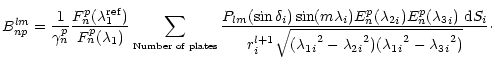
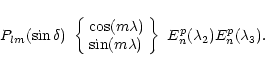
![$\displaystyle V(r,\delta,\lambda)=\mu~\sum_{l=0}^{\infty}\sum_{m=0}^{l}{1\over
r^{l+1}}~ P_{lm}(\sin\delta) [C_{lm}\cos(m\lambda)+S_{lm}\sin(m\lambda)]$](/articles/aa/full/2002/21/aa2371/img6.gif) |
(1) |
A&A 387, 1114-1122 (2002)
DOI: 10.1051/0004-6361:20020466
D. Dechambre - D. J. Scheeres
Department of Aerospace Engineering, The University of Michigan, Ann Arbor, MI 48109-2140
Received 13 February 2002 / Accepted 8 March 2002
Abstract
Analytical expressions linking spherical harmonics gravity field expansions with ellipsoidal harmonics
gravity field expansions are developed. Certain symmetries and simplifications for the transformation between the
two are noted. Using the expressions, a numerical approach is developed and applied for the computation of
ellipsoidal harmonic gravity coefficients using spherical harmonics coefficients as inputs. This method can be
used to transform a measured spherical harmonic gravity field into an ellipsoidal harmonic gravity field for use within the
Brillouin sphere of the original body. This would allow for the computation of spacecraft and natural trajectories close to
the surface of an asteroid or comet using a measured gravity field.
Key words: comets: general - gravitation - minor planets, asteroids
Small solar system bodies like asteroids and comets have become the target of current and forthcoming space missions. These bodies are known to have irregular shapes and complex gravity fields which can cause large perturbations to the trajectories of natural and artificial satellites in their vicinity. Thus, the measurement and use of a body's gravity field is of fundamental importance to understanding the environment close to its surface.
The classical approach for representing the gravitational field of an arbitrary body consists of expanding its gravitational potential into spherical harmonics (Kaula 1966). The distributed mass of the body is then modeled by the spherical harmonic coefficients Clm and Slm. These coefficients can be determined to high accuracy by evaluating the perturbations induced by the body on a spacecraft trajectory over the orbital phase of its mission. The advantage of this method is that it involves simple mathematics and converges to the correct gravity field outside the circumscribing (Brillouin) sphere about the body. In addition, finite truncations are often sufficient to match the "true potential'' of the body with good accuracy. Their drawback is that spherical harmonics expansions can exhibit severe divergence inside the circumscribing sphere. Thus they are not adequate to model the asteroid's gravity at close range.
Another approach consists of modeling the asteroid gravity field as a constant density polyhedron (Werner & Scheeres 1997). Small details of the asteroid surface can be included by modeling these regions with high resolution. The main advantage of this method is that the polyhedral potential is valid and exact for any given shape and density up to the surface of the body. Errors are thus reduced entirely to the errors in the asteroid shape determination and discretization. For Asteroid 433 Eros, a polyhedron model with 8200 plates was used to analyze close flybys of the surface (Antreasian et al. 1999). Despite the exactitude of the polyhedral potential, the constant density assumption can lead to erroneous gravity computations at close range. Improvements to match the "true gravity field'' more closely can be made by simulating density variations within the asteroid (Scheeres et al. 2000) but do not give a unique density distribution assignment. Thus, this approach cannot be used to develop a precision model of a body's gravitational field.
A third option for modeling a gravity field is the use of ellipsoidal harmonics (Garmier & Barriot 2001). While these harmonics still diverge when close to the body, their Brillouin ellipsoid lies much closer to the surface of the body. A disadvantage of the ellipsoidal harmonics is their complicated computation and the attendent difficulty to directly estimate these coefficients. Additionally, the estimation of spherical harmonic coefficients has been perfected to a high degree of accuracy, and thus one does not like to abandon their use altogether. To combine these approaches we propose a method for the transformation of measured spherical harmonic coefficients to an equivalent set of ellipsoidal harmonic coefficients. These gravity field expansions will then agree outside the Brillouin sphere of the body, and the ellipsoidal coefficients will be useable for computation of the gravity field within this sphere (but still outside of the Brillouin ellipsoid).
We first present the theory of ellipsoidal harmonics, introducing the ellipsoidal coordinates system and the Lamé functions. This theory was first developed by Byerly (1893), MacMillan (1930) and Hobson (1955), and was more recently applied by Garmier & Barriot (2001). The body of the paper describes a method for computing ellipsoidal harmonics directly from spherical harmonics. An analytical expression relating the ellipsoidal coefficients to the spherical coefficients is established. This result leads to a number of symmetry relations between ellipsoidal and spherical harmonic coefficients, and motivates the development of a numerical technique for transformation of spherical harmonic coefficients to ellipsoidal harmonic coefficients. Finally, numerical results are used to verify the cogency of our theory.
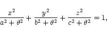
The gravitational potential V of an arbitrary body can be expanded in a spherical harmonics expansion as:
 |
(2) |
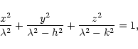
Similarly, the potential V can be expressed as a series of ellipsoidal harmonics involving the set of ellipsoidal coordinates
![]() .
.
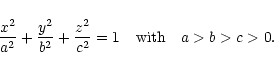
Ellipsoidal coordinates can be related in various ways to the Cartesian
coordinates. They are defined with respect to a fundamental ellipsoid of
semi-axes (a,b,c):
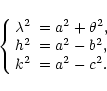 |
(6) |
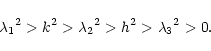
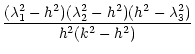
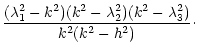
According to Eq. (5), there are eight points in space corresponding to the same
![]() .
These points are defined by
.
These points are defined by
![]() in
Cartesian
coordinates. Cartesian coordinates can be related to ellipsoidal coordinates using the following transformation:
in
Cartesian
coordinates. Cartesian coordinates can be related to ellipsoidal coordinates using the following transformation:
In the following, we will deal with spaces whose boundaries are ellipsoids and
solutions to Laplace's equation within these spaces. It is then convenient to
express Laplace's equation
![]() in terms of the ellipsoidal coordinates
in terms of the ellipsoidal coordinates
![]() .
.
In the othogonal set of coordinates
![]() ,
Laplace's
equation takes the form:
,
Laplace's
equation takes the form:
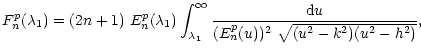
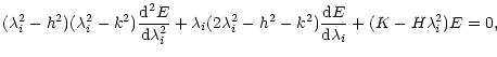
The parameters H and K can be chosen such that solutions to (11) take the general form:
 |
(12) |
 |
(13) |
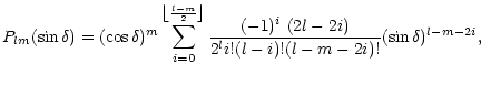
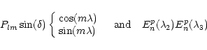
There are four types of Lamé functions of the first kind K, L, M and N defined according to the form of
the leading product ![]() .
.
Let us define ![]() as:
as:
 |
(14) |
-
![]() functions Enp of type K,
functions Enp of type K,
![]() ,
defined by:
,
defined by:
The Lamé products
![]() and
and
![]() are both normal solutions to
Lamé's Eq. (11). The former is continuous
within any ellipsoid
are both normal solutions to
Lamé's Eq. (11). The former is continuous
within any ellipsoid
![]() .
The latter is continuous
for
.
The latter is continuous
for
![]() and it vanishes when
and it vanishes when
![]() .
.
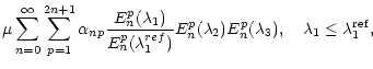
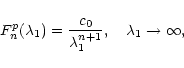
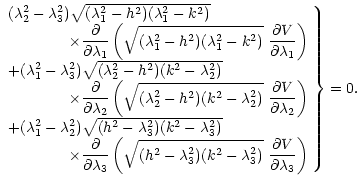
We can then define the ellipsoidal harmonics expansion of the potential anywhere in space as:
The indices (l,m) and (n,p) are called degree and order of the spherical harmonics expansion, respectively ellipsoidal harmonics expansion. For a given degree l=n, there are as many spherical harmonics (2l+1) as ellipsoidal harmonics (2n+1). Furthermore, there is a strong analogy in the expressions of the harmonics themselves that we will discuss in the followings.
When ![]() is very large,
is very large,
 |
(22) |
 |
(23) |
Similarly, one can relate the terms
 |
(24) |
The explicit parallelism between both expansions leads us to investigate
any relation between the ellipsoidal harmonics coefficients,
![]() ,
and the spherical harmonics coefficients, Clm and
Slm.
This will be the object of the next section.
,
and the spherical harmonics coefficients, Clm and
Slm.
This will be the object of the next section.
In the following, we want to express the normalized ellipsoidal harmonics
coefficients,
![]() ,
as a function of the spherical harmonics coefficients Clm and Slm.
,
as a function of the spherical harmonics coefficients Clm and Slm.
One can show, using Green's theorem, that the Lamé functions of the first kind satisfy the following relation:
Applying (25) to both sides of (21) yields:
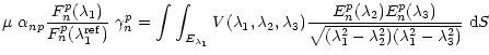 |
(26) |
Consider the term
 |
(31) |
Consider now the other term,
 |
(32) |
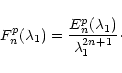
We will treat as an example the case where n is even,
![]() .
For
all the other cases, we will summarize the results in a table.
.
For
all the other cases, we will summarize the results in a table.
| l and m even | l and m odd | l even and m odd | l odd and m even | |||||||
| sign of Eq. | sign of Eq. | sign of Eq. | sign of Eq. | |||||||
| Pi |
|
|
|
|
|
|
|
|
|
|
| P1 | + | + | + | + | + | + | + | + | ||
| P2 |
|
+ | - | - | + | - | + | + | - | |
| P3 |
|
+ | + | - | - | - | - | + | + | |
| P4 |
|
+ | - | + | - | + | - | + | - | |
| P5 | + | + | + | + | - | - | - | - | ||
| P6 |
|
+ | - | - | + | + | - | - | + | |
| P7 |
|
+ | + | - | - | + | + | - | - | |
| P8 |
|
+ | - | + | - | - | + | - | + | |
We are here going to discuss the sign of
| type | n even | n odd | ||||||
| of | l even | l odd | l even | l odd | ||||
| Enp | m even | m odd | m even | m odd | m even | m odd | m even | modd |
| K | x | 0 | 0 | 0 | 0 | 0 | 0 | x |
| L | 0 | 0 | 0 | 0 | 0 | 0 | 0 | 0 |
| M | 0 | x | 0 | 0 | 0 | 0 | x | 0 |
| N | 0 | 0 | 0 | 0 | 0 | 0 | 0 | 0 |
| type | n even | n odd | ||||||
| of | l even | l odd | l even | l odd | ||||
| Enp | m even | m odd | m even | m odd | m even | m odd | m even | modd |
| K | 0 | 0 | 0 | 0 | 0 | 0 | 0 | 0 |
| L | x | 0 | 0 | 0 | 0 | 0 | 0 | x |
| M | 0 | 0 | 0 | 0 | 0 | 0 | 0 | 0 |
| N | 0 | x | 0 | 0 | 0 | 0 | x | 0 |
Let us distinguish the four cases:
 |
(35) |
By going through all the cases individually, we obtain the following tables for the
Anplm and
Bnplm.
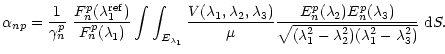
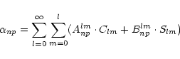
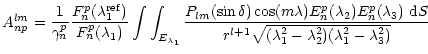
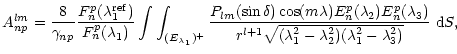
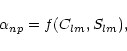
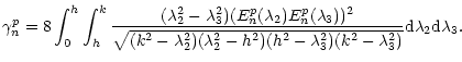
Using Tables 2 and 3, the relation between ellipsoidal harmonics coefficients and spherical harmonics coefficients can be simplified. Depending on the values of the degree n and the order p, Eq. (28) reduces to:
| = | (36) | ||
| = | (37) | ||
| = | (38) | ||
| = | (39) |
| = | (40) | ||
| = | (41) | ||
| = | (42) | ||
| = | (43) |
When considering an attracting body, the spherical harmonics expansion of the potential is uniformly convergent
outside the Brillouin sphere. The Brillouin sphere is defined as the smallest sphere that encloses the attracting
body. Inside the Brillouin sphere, severe divergences of the spherical harmonics expansion may occur.
Similary, the ellipsoidal harmonics expansion of the potential is uniformly convergent outside the Brillouin ellipsoid. The
Brillouin ellipsoid is defined as the smallest ellipsoid that encloses the attracting body. Inside the Brillouin
ellipsoid, severe divergences of the ellipsoidal harmonics expansion may occur.
In Sect. 3.1, the linear transformation (28),
 |
(44) |
Ellipsoidal harmonics are more appropriate than spherical harmonics to compute the gravity field of irregularly shaped attracting bodies. Since an arbitrary shape body is better fitted by an ellipsoid than by a sphere, the region of divergence of an ellipsoidal harmonics expansion is smaller than the one of a spherical harmonics expansion (see paragraph 3.2.3).
In the following, we are going to use the
method described above for the evaluation of the ellipsoidal coefficients
![]() .
Given spherical
coefficients Clm and Slm, we are then going to "reconstruct'' the corresponding spherical harmonics
expansion of the potential with an ellipsoidal harmonics expansion.
.
Given spherical
coefficients Clm and Slm, we are then going to "reconstruct'' the corresponding spherical harmonics
expansion of the potential with an ellipsoidal harmonics expansion.
Expression of the potential in Eq. (21) requires the knowledge of the ellipsoidal coefficients
![]() ,
the Lamé functions of the first and second kind and the ellipsoidal coordinates.
,
the Lamé functions of the first and second kind and the ellipsoidal coordinates.
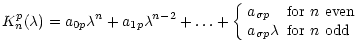
Lamé functions of the first kind Enp have explicit expressions up to n=3. For n>3, Ritter and Dobner have
transformed the problem of computing the polynomial coefficients in Eqs. (15), (16),
(17) and (18) into an eigenvalue problem (see Ritter 1998 and Dobner & Ritter 1998). Regarding
Lamé functions of the second kind Fnp defined by (19), they can be evaluated numerically using a
Gauss-Legendre quadrature (see Garmier & Barriot 2001).
The ellipsoidal coordinates
![]() have been defined as the roots of Eq. (5). They
can be explictly expressed in terms of the Cartesian coordinates (x,y,z). However these solutions may be
singular and we rather use a numerical solver such as a false position method (see Press et al. 1993) to determine
the roots of (5).
have been defined as the roots of Eq. (5). They
can be explictly expressed in terms of the Cartesian coordinates (x,y,z). However these solutions may be
singular and we rather use a numerical solver such as a false position method (see Press et al. 1993) to determine
the roots of (5).
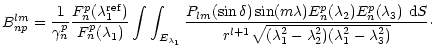
Finally, the ellipsoidal coefficients
![]() have been constructed from the spherical coefficients Clmand Slm by the linear transformation (28). We have seen in Sect. 3.2 that
the coefficients
Anplm and
Bnplm vanish in many cases. However, when a priori non zero, no
explicit expression exists. Instead, we "tessellate'' the surface of the ellipsoid
have been constructed from the spherical coefficients Clmand Slm by the linear transformation (28). We have seen in Sect. 3.2 that
the coefficients
Anplm and
Bnplm vanish in many cases. However, when a priori non zero, no
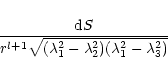
explicit expression exists. Instead, we "tessellate'' the surface of the ellipsoid
![]() into flat
triangular faces (Fig. 1). The vertices of theses faces are placed on the surface of the
ellipsoid with constant latitude and longitude increments. To first approximation, the integrands in expressions (29) and (30) are treated as constant over each plate so that the integral over the
surface
into flat
triangular faces (Fig. 1). The vertices of theses faces are placed on the surface of the
ellipsoid with constant latitude and longitude increments. To first approximation, the integrands in expressions (29) and (30) are treated as constant over each plate so that the integral over the
surface
![]() is transformed into a finite summation over the number of plates:
is transformed into a finite summation over the number of plates:
 |
(47) |
![\begin{figure}
\par\includegraphics[width=8cm,clip]{ms2371sf1.eps}\end{figure}](/articles/aa/full/2002/21/aa2371/img129.gif) |
Figure 1:
"Tessellated surface'' of the ellipsoid
|
| Open with DEXTER | |
In the following, we focus on the computation of the external gravity field for asteroid 433 Eros (Yeomans et al. 2000). We assume the knowledge of the spherical coefficients Clm and Slm for Eros. They completely describe the spherical gravity field of the asteroid. Using Eqs. (21) and (28), we will compute the ellipsoidal harmonics expansion for Eros. We will then compare the resulting ellipsoidal gravity field with the given spherical gravity field. We expect them to match outside the Brillouin sphere where spherical and ellipsoidal harmonics expansions are both convergent.
The Brillouin ellipsoid is defined as the ellipsoid that best fits the asteroid. In Eqs. (20) and (21), we choose
![]() equal to the semi-major axis of the Brillouin ellipsoid. With this
choice of
equal to the semi-major axis of the Brillouin ellipsoid. With this
choice of
![]() ,
(20) and (21) respectively define the interior and the exterior
potential of the Brillouin ellipsoid. For our simulations, we choose a Brillouin ellipsoid for asteroid Eros of
semi-axes
,
(20) and (21) respectively define the interior and the exterior
potential of the Brillouin ellipsoid. For our simulations, we choose a Brillouin ellipsoid for asteroid Eros of
semi-axes
![]() and a Brillouin sphere of radius
and a Brillouin sphere of radius
![]() .
These data are computed from a discretized shape model of the surface of the asteroid.
.
These data are computed from a discretized shape model of the surface of the asteroid.
Per Sect. 3.2.3, the "tesselated'' ellipsoid
![]() used for the numerical
evaluation of the ellipsoidal coefficients
used for the numerical
evaluation of the ellipsoidal coefficients
![]() must be chosen such that it encloses the Brillouin
sphere. In order to minimize the error between its "tesselated'' surface and its "true'' surface, we choose for
must be chosen such that it encloses the Brillouin
sphere. In order to minimize the error between its "tesselated'' surface and its "true'' surface, we choose for
![]() the smallest ellipsoid confocal to the Brillouin ellipsoid that encloses the Brillouin sphere: its
semi-axes are
the smallest ellipsoid confocal to the Brillouin ellipsoid that encloses the Brillouin sphere: its
semi-axes are
![]() .
.
![\begin{figure}
\par\includegraphics[width=8cm,clip]{ms2371sf2.eps}\end{figure}](/articles/aa/full/2002/21/aa2371/img134.gif) |
Figure 2: Maximum error on the computation of the potential for Eros. |
| Open with DEXTER | |
![\begin{figure}
\par\includegraphics[width=8cm,clip]{ms2371sf3.eps}\end{figure}](/articles/aa/full/2002/21/aa2371/img135.gif) |
Figure 3: Weighted error on the computation of the potential for Eros. |
| Open with DEXTER | |
![\begin{figure}
\par\includegraphics[angle=90,width=10cm,clip]{ms2371sf4.eps}\end{figure}](/articles/aa/full/2002/21/aa2371/img136.gif) |
Figure 4:
Errors
|
| Open with DEXTER | |
Given a spherical harmonics expansion of degree 6 (Clm and Slm up to l=6), we compute the ellipsoidal
potential ![]() for various degrees n of the ellipsoidal harmonics expansion up to n=12. We then evaluate the
error
for various degrees n of the ellipsoidal harmonics expansion up to n=12. We then evaluate the
error ![]() between
between ![]() and the spherical potential of degree 6 taken as the reference,
and the spherical potential of degree 6 taken as the reference,
![]() :
:
 |
(48) |

The error ![]() is plotted on Figs. 2 and 3 for three "tesselated''
surface models of
is plotted on Figs. 2 and 3 for three "tesselated''
surface models of
![]() :
:
Differentiating Eqs. (1) and (21) with respect to x, y and z, one can obtain the
expressions of the spherical and ellipsoidal accelerations vectors. The ellipsoidal acceleration components can be
analytically written as:
| = | ![$\displaystyle \mu\sum_{n=0}^{\infty}\sum_{p=1}^{2n+1}{\alpha_{np}\over
F_n^p\le...
...\partial\lambda_1}-{2n+1\over
\sqrt{(\lambda_1^2-h^2)(\lambda_1^2-k^2)}}\right]$](/articles/aa/full/2002/21/aa2371/img151.gif) |
||
 |
(49) |
With the model described in Sect. 4.2, we evaluated the errors
![]() ,
,
![]() and
and
![]() between the components of the ellipsoidal acceleration of degree n and the
components of the spherical acceleration of degree 6 taken as a reference defined as:
between the components of the ellipsoidal acceleration of degree n and the
components of the spherical acceleration of degree 6 taken as a reference defined as:
 |
(50) |
Ellipsoidal harmonics are useful for the representation of asteroid and comet gravity fields.
Our approach is to use our knowledge of spherical harmonics to provide a better understanding of the ellipsoidal
harmonics theory. Because of the obvious analogies between spherical and ellipsoidal harmonics, we have been interested in
establishing an analytical expression that relates the ellipsoidal harmonic coefficients
![]() to the
spherical harmonic coefficients Clm and Slm. Though no explicit formulation exists for Eq. (28), we have shown that it can be further simplified based on symmetry arguments and can be used to develop a
numerical transformation procedure. Plots have been provided to validate the computation of ellipsoidal harmonics using
spherical harmonics.
to the
spherical harmonic coefficients Clm and Slm. Though no explicit formulation exists for Eq. (28), we have shown that it can be further simplified based on symmetry arguments and can be used to develop a
numerical transformation procedure. Plots have been provided to validate the computation of ellipsoidal harmonics using
spherical harmonics.

![$\displaystyle L_n^p(\lambda)=\sqrt{\vert\lambda^2-h^2\vert} \bigg[b_{0p}\lambda...
... even}\\
b_{{n-\sigma-1},p} &\hbox{for $n$\space odd}\end{array} \right.\bigg]$](/articles/aa/full/2002/21/aa2371/img44.gif)
![$\displaystyle M_n^p(\lambda)=\sqrt{\vert\lambda^2-k^2\vert} \bigg[c_{0p}\lambda...
... even}\\
c_{{n-\sigma-1},p} &\hbox{for $n$\space odd}\end{array} \right.\bigg]$](/articles/aa/full/2002/21/aa2371/img46.gif)
![$\displaystyle N_n^p(\lambda)=\sqrt{\vert(\lambda^2-h^2)(\lambda^2-k^2)\vert}\bi...
...}\\
d_{{\sigma-1},p}\lambda &\hbox{for $n$\space odd}\end{array}\right.\bigg].$](/articles/aa/full/2002/21/aa2371/img48.gif)