A&A 387, L25-L28 (2002)
DOI: 10.1051/0004-6361:20020509
Search for decametric occultations of Io flux tube by Ganymede
A. V. Arkhipov (O. V. Arkhypov)
Institute of Radio Astronomy, Nat. Acad. Sc. of Ukraine,
Chervonopraporna 4, 61002 Kharkiv, Ukraine
Received 5 December 2001 / Accepted 2 April 2002
Abstract
The satellite Ganymede sometimes occults the sources of the Jovian
decameter radiation (DAM) associated with Io magnetic field line.
The basic parameters of Ganymede occultations are calculated for
1990-2010. One of these events is found to coincide with a Io-A
radio storm, which has been recorded in Nancay Observatory on 17 April 1994. In spite of the difficulty to identify the satellite
shadow on sporadic DAM, the ratio of frequency emitted to
calculated gyromagnetic frequency of electrons in the source is
tentatively estimated as
 .
Formally, this limit contradicts the present generation
theories where
.
Formally, this limit contradicts the present generation
theories where
 in the DAM source is much closer
to 1. Hence, improvements to the magnetic model (VIP4) or of the
distortion of the Io flux tube are needed. Two possible shadows of
the satellite are tentatively identified on the DAM frequency-time
spectrogram. Multiple occultations are indeed possible in the
Alfven wave model of Io-DAM interaction, and the lead angle of the
emitting field line is not well known. That is why the tentative
location of the radio source is made for both variants.
in the DAM source is much closer
to 1. Hence, improvements to the magnetic model (VIP4) or of the
distortion of the Io flux tube are needed. Two possible shadows of
the satellite are tentatively identified on the DAM frequency-time
spectrogram. Multiple occultations are indeed possible in the
Alfven wave model of Io-DAM interaction, and the lead angle of the
emitting field line is not well known. That is why the tentative
location of the radio source is made for both variants.
Key words: planets and satellites: individual -
occultations -
magnetic fields -
radiation mechanisms: non-thermal
It has been shown that the Galilean satellites can eclipse the
sources of the Jovian decameter radiation (DAM) (Arkhipov
1997, 2001). Such occultations could
help to precisely localize the regions of DAM generation and
reveal the fine structure of the DAM sources. Moreover, the ratio
of emission frequency to local cyclotron frequency of electrons in
the source could be measured and used for evaluation of DAM
theories.
The occultation method had been applied to the Jovian radio
emissions only during the Galileo mission, at short distances and
low frequencies ( 5.6 MHz; Kurth et al.
1997). In this way, new information could be obtained from
Earth based observations.
5.6 MHz; Kurth et al.
1997). In this way, new information could be obtained from
Earth based observations.
That is why archive searches for DAM eclipses as well as new
observations are very desirable. For this task the basic
parameters of Ganymede occultations are calculated in this
article.
In accordance with present ideas on the radio emission generation,
the following model is assumed for occultation calculations.
Jovian decameter radio emission is generated in fast extraordinary
mode just above the local cyclotron frequency of electrons (
)
(see e.g. Zarka 1998). Even if
 ,
refraction probably becomes negligible at a short
distance from the source, so that straight line propagation is an
acceptable approximations for simplification of calculations. Of
course, f could be significantly above
(it is
unknown a priori). However, our
,
refraction probably becomes negligible at a short
distance from the source, so that straight line propagation is an
acceptable approximations for simplification of calculations. Of
course, f could be significantly above
(it is
unknown a priori). However, our
 approximation is still a useful asymptotic marker for prediction
and practical search for occultations.
approximation is still a useful asymptotic marker for prediction
and practical search for occultations.
The Io-controlled emission is generated along or close to the
magnetic field line connected with Io (Io flux tube - IFT; Fig. 1)
(Carr et al. 1983). This IFT is calculated as an
undisturbed magnetic line according to the VIP-4 model (Connerney
et al. 1998). Of course, some delay of Io-Jupiter
interaction must be taken into consideration. Thus the radio
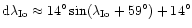
emitting field line is traced, which is formally connected with
"effective''position of Io in the satellite orbital plane, at
jovigraphic longitude
 ,
where:
,
where:
 is the
true Io longitude; and
is the
true Io longitude; and
 is the
lead angle. Here the corrections
are supposed with the two alternative
methods:
is the
lead angle. Here the corrections
are supposed with the two alternative
methods:
(a) as approximation of difference between orbital longitudes
and the Io effective position, deduced
from UV observations of IFT footprints (Clarke
1996):
 (north);
 (south). Uncertainty on the lead angle is of the order of
several degrees.
(south). Uncertainty on the lead angle is of the order of
several degrees.
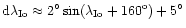
(b) according to the analysis of DAM radiation pattern (Queinnec
& Zarka 1998),
 (north) or
  (south) has been
adopted.
(south) has been
adopted.
This dual strategy is reasonable, because the lead angle may be
different in radio and UV, as the emitting electrons may not be
exactly the same populations. As a result, the position of an
Io-controlled DAM source is calculated as a point with
on the magnetic line, which is connected with
Io's effective position.
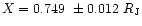
The geocentric, differential coordinates of Jovian satellites are
calculated with interpolation of ephemerides from Bureau des
longitudes (www.bdl.fr/ephem/ephesat/satformbis.html). Although
the errors of calculated positions are 0.001
 (
(
 is the equatorial radius
of Jupiter), the real precision of eclipse prediction is limited
by the lead angle uncertainty. Practically the error in visible
coordinate of source is about the diameter of Ganymede (0.074
).
is the equatorial radius
of Jupiter), the real precision of eclipse prediction is limited
by the lead angle uncertainty. Practically the error in visible
coordinate of source is about the diameter of Ganymede (0.074
).
![\begin{figure}
\par\includegraphics[width=8.8cm,clip]{DL051_F1.EPS}
\end{figure}](/articles/aa/full/2002/20/aadi051/Timg21.gif) |
Figure 1:
Scheme of an occultation of the Io flux tube
by Ganymede. |
| Open with DEXTER |
To plan and analyze the observations, all IFT occultations by
Ganymede have been calculated for 1990-2010 (see Table 1).
Sometimes the Ganymede's centre occults IFT only with the UV lead
angle, while it is impossible with the radio angle and vice versa.
The following information is tabulated there for both versions (a)
and (b) of lead angle: the date of occultation (day/month/year);
the universal time of the event (UT; hour, min.); the frequency of
the shadow center in dynamical spectrum of DAM (MHz); the central
meridian longitude of Jupiter at occultation (CML, degree in
system III 1965); the Io phase at occultation (
 ,
degree;); the hemisphere of occulted source (N- north; S- south);
the geographical longitude (
,
degree;); the hemisphere of occulted source (N- north; S- south);
the geographical longitude (
 ,
degree); and
latitude (
,
degree); and
latitude (
 ,
degree) of sub-Jovian point on
the Earth at occultation.
,
degree) of sub-Jovian point on
the Earth at occultation.
To estimate the visibility of Jupiter for any observatory, the
zenith angle of Jupiter could be calculated
![\begin{displaymath}Z_{{\rm obs}} =\arccos [ \sin \varphi_{{\rm j}}
\sin \varphi...
...rphi_{{\rm o}} \cos (\lambda_{{\rm o}} -
\lambda_{{\rm j}})]
\end{displaymath}](/articles/aa/full/2002/20/aadi051/img25.gif) |
(1) |
where:
 and
and
 are
the longitude and latitude of the observatory.
are
the longitude and latitude of the observatory.
Obviously, such occultation is observable when a satellite
eclipses the active DAM source, emitting towards the Earth.
According to the maps of DAM occurrence for right- and left-hand
polarizations separately (Carr & Desh 1976; Boudjada &
Genova 1991), the most promising occultations are
asterisked.

The lead angle is taken from
UV data.

The lead angle is taken from radio
data.
![\begin{figure}
\par\includegraphics[width=7.5cm,clip]{DL051_F2.EPS}
\end{figure}](/articles/aa/full/2002/20/aadi051/Timg32.gif) |
Figure 2:
Probable IFT occultations on the DAM dynamical
spectrum of 17 April 1994 (right hand polarization). The predicted
shadow contours with
 and
and
 a) or
b) are shown as the light
ellipsoids on the left panel. The candidates in the Ganymedes
shadow are shown on the right panel: c)
a) or
b) are shown as the light
ellipsoids on the left panel. The candidates in the Ganymedes
shadow are shown on the right panel: c)
 and
and
 ;
d) ;
d)
 and
and
 . . |
| Open with DEXTER |
Unfortunately, no Jupiter observations were made on predicted
dates with the UTR-2 radio telescope of the Institute of Radio
Astronomy (Kharkov, Ukraine). The synoptic dynamic spectra of DAM
from the archives of Nancay Observatory (http://www.obs-nancay.fr/jupiter) have thus been used for the
occultation search. As Ganymede occults some part of an emitting
magnetic field line, the corresponding interval of frequencies
must be shadowed in the DAM dynamical spectrum. Thus an elongated
dark spot is formed in the spectrum, and this could be calculated.
The typical dimensions of such a spot are 10 min and 9 MHz.
All corresponding Nancay spectra have been analysed (28/01/1994;
17.04.1994; 24/04/1994; 28.09.1994; 12.02.1995; 25.08.2000). Only
on 17 April 1994 an Io-A storm (with right hand polarization) was
recorded just in the predicted time interval of occultation. Both
calculated contours of the Ganymede shadow, with the different
lead angles (a) and (b), overlap the L-emission (Fig. 2,
left). Of course, one possible explanation is the existence of
several simultaneous radio sources, out of which only one is
occulted by the satellite shadow. Conversely, there are two
possible identifications of Ganymedes shadow above the Io-storm
(Fig. 2, right). The most suitable ellipsoids are
calculated with
 and
and
 ,
and
,
and  for (c) and (d) contours respectively. The search for interference
fringes which should exist along the shadow borders (Arkhipov
2001) is impossible with the low resolution of the
published spectrum.
for (c) and (d) contours respectively. The search for interference
fringes which should exist along the shadow borders (Arkhipov
2001) is impossible with the low resolution of the
published spectrum.
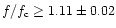
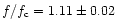
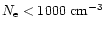
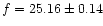
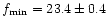
In spite of the recognition problem, the spectrum of 17 April 1994
is of interest. Thus,
for
any identification of the shadow in the most probable range
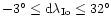 .
Formally, this limit contradicts the hypothesis
that
.
Formally, this limit contradicts the hypothesis
that
 in the DAM source is much closer to 1.
It is now believed (Zarka 1998) that DAM emission is
produced close to the X mode cutoff at
in the DAM source is much closer to 1.
It is now believed (Zarka 1998) that DAM emission is
produced close to the X mode cutoff at
![\begin{displaymath}f \sim f_{{\rm c}} [~ 1 + (f_{{\rm p}} /
f_{{\rm c}})^2 ~ ]
\end{displaymath}](/articles/aa/full/2002/20/aadi051/img38.gif) |
(2) |
where
 is the plasma
frequency of electrons and
is the plasma
frequency of electrons and
 is the electron
density. Hence
is the electron
density. Hence
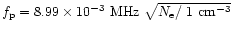
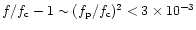 with
with
 and
and
 in the DAM source when extrapolated from Voyager 2 radio
occultation (Hinson et al. 1998).
The DAM polarization suggests
in the DAM source when extrapolated from Voyager 2 radio
occultation (Hinson et al. 1998).
The DAM polarization suggests
 in IFT (e.g.: Shaposhnikov et al.
2000). Therefore, the found limit
appears surprisingly high.
in IFT (e.g.: Shaposhnikov et al.
2000). Therefore, the found limit
appears surprisingly high.
It is difficult to explain this result in terms of exotic lead
angle (
 or
or
 ).
Apparently, the
derived from magnetic field
model could be underestimated. However, the gyromagnetic
frequency, calculated using VIP4 and previous O6 GSFC models, has
a quadratic difference of only 1.4 MHz along the Io magnetic shell
at planetocentric distance of the occultation (
).
Apparently, the
derived from magnetic field
model could be underestimated. However, the gyromagnetic
frequency, calculated using VIP4 and previous O6 GSFC models, has
a quadratic difference of only 1.4 MHz along the Io magnetic shell
at planetocentric distance of the occultation (
 ). Hence, the standard error on calculated
is <1 MHz with VIP4, while the storm border
exceeds the calculated
by >2.3 MHz. Another
explanation of this discrepancy may be due to the additional
magnetic field distortion by the electrical current which flows
along the Io flux tube.
). Hence, the standard error on calculated
is <1 MHz with VIP4, while the storm border
exceeds the calculated
by >2.3 MHz. Another
explanation of this discrepancy may be due to the additional
magnetic field distortion by the electrical current which flows
along the Io flux tube.
It has been strongly argued that Io-B DAM cannot arise from the
instantaneous IFT only (Leblanc et al. 1994; Queinnec &
Zarka 1998). It was proposed that the arcs of
Io-controlled DAM are caused by a pattern of field-aligned
currents, which are separated in longitude. These currents are
carried by the Alfvenic disturbances as they bounce between the
northern and southern ionospheres and the Io torus edge (e.g.:
Bagenal & Leblanc 1988). Apparently, there are two arcs
in the Io-A storm of 17 April 1994. Hence, a pair of radio sources
could cause two shadows in the dynamic spectrum. This also
justifies why both possible shadows are worth consideration.
The shadows border point with lowest frequency could be used
for localization of the occulted radio source without any
dependence upon the magnetic model. The universal time and
frequency of this point is found for (c) ellipsoid by parabolic
approximation of the storm border:
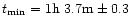 m and
m and
 MHz (arrowed in Fig. 2). The tangential coordinates of the radio source with
this frequency are:
MHz (arrowed in Fig. 2). The tangential coordinates of the radio source with
this frequency are:
where: the Y axis is directed from the center of Jupiter to its
northern pole;
 ,
,
 are the Ganymede
coordinates for
are the Ganymede
coordinates for
 ;
;
 is the Ganymedes radius. For (d) ellipsoid:
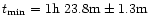 ;
;
 MHz;
MHz;
 ;
;
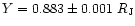 .
Of course, these coordinates are tentative.
.
Of course, these coordinates are tentative.
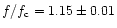
- 1.
- In 1990-2010 about 24 radio occultations of the Io flux
tube by Ganymede could be observed from the Earth. Such phenomena
are a promising and still unused tool to study the Jovian
magnetosphere.
- 2.
- One of this events coincided with the Io-A radio storm, which was
recorded in Nancay Observatory on 17 April 1994. The first attempt
to measure directly the ratio of frequency emitted to calculated
gyromagnetic frequency of electrons in the source leads to the
limit of
.
Formally, this
limit contradicts the hypothesis that
in the
DAM source is much closer to 1. One possible explanation is that
the occultation is actually "hidden'' by simultaneously emitting
nearby radio sources (with
 ).
Conversely, improvements to the magnetic model (VIP4) may be
needed; or/and the distorsion of the Io flux tube must be taken
into account.
).
Conversely, improvements to the magnetic model (VIP4) may be
needed; or/and the distorsion of the Io flux tube must be taken
into account.
- 3.
- Two candidate Ganymedes shadows are found on the DAM dynamic
spectrum of 17 April 1994. Multiple occultations could be
explained in terms of the Alfven wave model of Io-DAM interaction.
However, the obtained coordinates of sources are tentative.
- 4.
- New observations of IFT occultations by Ganymede are desirable in
2005-2006.
Acknowledgements
I would like to express many thanks to Dr. Ph. Zarka, Dr.
J. E. P. Connerney, Dr. J. H. Lieske, Dr. H. O. Rucker for their
help with the literature and consultations. I also wish to thank
Dr. L. Fleming for reading and commenting on the manuscript.
- Arkhipov, A. V. 1997, in Planetary Radio
Emissions IV, ed. H. O. Rucker, S. J. Bauer, & A. Lecacheux (Austrian
Academy of Sciences Press, Vienna), 129
In the text
- Arkhipov, A. V. 2001, in Planetary Radio
Emissions V, ed. H. O. Rucker, M. L. Kaiser, & Y. Leblanc (Austrian
Academy of Sciences Press, Vienna), 165
In the text
- Bagenal, F., & Leblanc, Y. 1988, A&A,
197, 311
In the text
NASA ADS
- Boudjada, M. Y., & Genova, F. 1991, A&AS,
91, 453
In the text
NASA ADS
- Carr, T. D., & Desh, M. D. 1976, in Jupiter,
ed. T. Gehrels (University of Arizona Press, Tucson), 693
In the text
- Carr, T. D., Desh, M. D., & Alexander, J. K. 1983,
in Physics of the Jovian Magnetosphere, ed. A. J. Dessler (Cambridge
Univ. Press, Cambridge), 226
In the text
- Clarke, J. T. 1996, Science, 274, 404
In the text
NASA ADS
- Connerney, J. E. P., Acuña, M. H., Ness, N. F., & Satoh, T. 1998, J. Geoph.
Res., 103, A6, 11929
In the text
- Hinson, D. P., Twicken, J. D., & Karayel,
E. T. 1998, J. Geophys. Res., 103, 9505
In the text
NASA ADS
- Kurth, W. S., Bolton, S. J., Gurnett, D. A., & Levin, S. 1997, Geophys. Res. Lett.,
24, 1171
In the text
- Leblanc, Y., Dulk, G. A., & Bagenal, F.
1994, A&A, 290, 2, 660
In the text
NASA ADS
- Queinnec, J., & Zarka, P. 1998, J.
Geophys. Res., 103, A11, 26649
In the text
- Shaposhnikov, V. E., Rucker, H. O.,
& Zaitsev, V. V. 2000, A&A, 355, 2, 804
In the text
NASA ADS
- Zarka, P. 1998, J. Geophys. Res., 103,
20159
In the text
Copyright ESO 2002
![\begin{figure}
\par\includegraphics[width=8.8cm,clip]{DL051_F1.EPS}
\end{figure}](/articles/aa/full/2002/20/aadi051/img21.gif)
![\begin{figure}
\par\includegraphics[width=7.5cm,clip]{DL051_F2.EPS}
\end{figure}](/articles/aa/full/2002/20/aadi051/img32.gif)