A&A 387, 339-346 (2002)
DOI: 10.1051/0004-6361:20020302
D. A. Diver1 - A. A. da Costa 2 - E. W. Laing 1
1 - Dept of Physics and Astronomy, University of Glasgow, Glasgow G12 8QQ, Scotland, UK
2 -
Centro de Electrodinâmica, Instituto Superior Técnico, 1049-001 Lisboa, Portugal
Received 12 December 2001 / Accepted 27 February 2002
Abstract
The electron-positron plasma present in pulsar
magnetospheres may have non-linear electrostatic oscillations,
which can couple to electromagnetic waves if the magnetic field
present is inhomogeneous. Using a cylindrical geometry the basic
equations are derived, and using a simplified linear approach
characteristic linear modes are identified and analysed. A
possible coupling mechanism is discussed, and possible
consequences for pulsar radiation mechanisms are inferred.
Key words: plasmas - radiation mechanisms: non-thermal - pulsars: general
In a previous paper (da Costa et al. 2001, hereafter referred as Paper I) it was shown that the motion of equal-mass plasma in pulsar magnetospheres required the consideration of non-linear effects in the rest frame of the plasma. Within the context of cold plasmas, the non-linear electron-positron oscillation exhibits a density instability, in which the number density of each species grows sharply at the edges of the confined oscillation. Such a phenomenon is unphysical since ultimately annihilation will result.
There are several possible mechanisms which may quench this instability, such as pressure effects which would inhibit density growth. In this paper an investigation into the coupling of electrostatic and electromagnetic modes has been initiated, in which electrostatic perturbations trigger electromagnetic radiation. Such a coupling is desirable for two reasons: not only would it limit the energy in the oscillation by radiating it away, it could also act as a seat of radiation in a pulsar environment.
This mechanism is consistent with other forms of indirect radiation mechanisms, where primary effects generate secondary electromagnetic effects (Melrose 1993; Asseo & Melikidze 1998; Melikidze et al. 2000; Asseo & Riazuelo 2000). There are however two main differences.
First, this is no longer a pure dynamical process
in the laboratory frame of the pulsar, but one in the rest frame
of the plasma translated in the laboratory frame, as suggested by
Melrose (2000). Due to the quasi-static nature of the phenomena in
pulsar magnetospheres where the azimuthal dependence is given by
![]() ,
this is a real lighthouse effect
which when sitting outside the speed of light cylinder will have
superluminal characteristics (da Costa & Kahn 1985; Ginzburg
1989).
,
this is a real lighthouse effect
which when sitting outside the speed of light cylinder will have
superluminal characteristics (da Costa & Kahn 1985; Ginzburg
1989).
Second, the primary process is not strictly thermal, as seen in Paper I, but it might be a stochastic perturbation induced in the rest frame either directly by the quasi-classical process as described by da Costa & Kahn (1997), or other possible phenomena, as the presence of complex non-thermal plasma density distribution functions which will act to produce non-thermal phenomena similar to the one described by Asseo & Melikidze (1998).
The present paper addresses the basic mathematical formulation of the electron-positron (E-P) cold magnetoplasma connection between electrostatic and electromagnetic modes in Sect. 2, in the rest frame of the initially unperturbed magnetoplasma. It then proceeds in Sect. 3 to formulate the numerical algorithm designed specifically to solve the problem. Results are also presented here, and are discussed in Sect. 4. Finally, the implications for future research are analysed in Sect. 5.
In Paper I the non-linear oscillations of an unmagnetized E-P plasma were studied. However in order to couple the electrostatic mode to propagating electromagnetic radiation a non-uniform magnetic field is required, and therefore oscillations in an E-P magnetoplasma have to be considered.
Given that the propagation of an electromagnetic wave from a confined electrostatic oscillation is intrinsically a two-dimensional phenomenon, the one-dimensional treatment of the e+e- oscillation as considered in Paper I has to be extended. The simplest possible geometry is cylindrical, in which the oscillations are assumed radial, and the electromagnetic behaviour involves an axial magnetic perturbation and an azimuthal electric field.
Using the cylindrical geometry (
![]() )
in which the magnetic field
)
in which the magnetic field
![]() is only axial, the electric field
is only axial, the electric field ![]() lies in the
lies in the ![]() -plane and all
plasma variables depend only on r and t. The
full non-linear model equations are then (for a cold electron-positron plasma)
-plane and all
plasma variables depend only on r and t. The
full non-linear model equations are then (for a cold electron-positron plasma)
This non-linear system of equations does not have a closed form
analytical solution, and the electrostatic and electromagnetic
modes are mixed. In this preliminary investigation only the normal
modes arising from the linearised equations are considered in
order to identify a simple mechanism for cross-coupling between
electrostatic and electromagnetic behaviour. The linearised
equations can be cast in non-dimensional form as
| (20) | ||
| (21) |
| (22) | |||
| (23) | |||
| (24) | |||
| (25) | |||
| (26) | |||
| (27) | |||
| (28) | |||
| (29) | |||
| (30) |
| (31) | |||
| (32) | |||
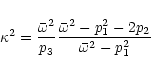
| p3=c2T2/R2 | (33) | ||
| (34) | |||
| (35) |
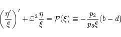
The electrostatic oscillation is characterised by Bz=B0, a
constant, requiring
![]() ,
the latter condition removing the
possibility of an undesirable non-zero time-invariant azimuthal
electric field. Hence
,
the latter condition removing the
possibility of an undesirable non-zero time-invariant azimuthal
electric field. Hence ![]() ,
,
![]() ,
implying b=d and a=-c.
On substitution into Eqs. (11)-(19) the equation
for
,
implying b=d and a=-c.
On substitution into Eqs. (11)-(19) the equation
for ![]() is obtained:
is obtained:
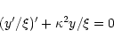
| (36) |
| (37) |
 |
(38) |
 |
(39) |
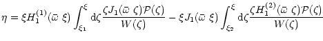
The physical mechanism behind the oscillation is as follows. A positive radial electric field (for example) causes electrons to move radially inward, and positrons radially outward, from their rest positions. Hence a=-c. Each particle however is deflected by the axial magnetic field, executing a partial Larmor orbit with the same azimuthal velocity; hence b=d. The resulting charge separation produces a restoring force causing the particles to return to their initial positions, but overshoot. However, the characteristic time taken to retrace their trajectories depends on the strength of the accelerating electric field (via the number density) and also on the magnetic curvature. The electrostatic oscillation here then is a radial expansion plus torsional twist, similar to the dynamics of a watch-spring.
When
Bz=Bz(r,t), an electromagnetic wave is present with an
azimuthal electric field component
![]() .
This
gives a radially radiating mode. Hence
.
This
gives a radially radiating mode. Hence
| |
= | (40) | |
| = | (41) |
| (42) |
| (43) | |||
| (44) |
![\begin{displaymath}\theta\propto\sqrt{\xi}\exp\left[i\left(\kappa\xi-\bar{\omega}\tau\right)\right]
\end{displaymath}](/articles/aa/full/2002/19/aah3345/img74.gif) |
(48) |
![\begin{displaymath}E_\theta\propto\theta/\xi\propto\xi^{-1/2}\exp\left[i\left(\kappa\xi-\bar{\omega}t\right)\right].
\end{displaymath}](/articles/aa/full/2002/19/aah3345/img75.gif) |
(49) |
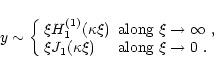
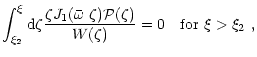
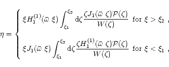
Summarizing, assuming the medium to be an unbounded, constant density plasma with a uniform equilibrium magnetic field, the electromagnetic mode in its simplest state propagates radially and has an azimuthal electric field, and an axial magnetic field. The "wavelength'' of the mode is determined by the behaviour of the Hankel function H(1)1, and its dispersion relation is given by (46).
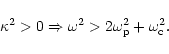
There are two normal modes: a pure electrostatic oscillation, in
which ![]() ,
a=-c, b=d,
,
a=-c, b=d, ![]() and
and
![]() ;
and a pure electromagnetic
mode, for which
;
and a pure electromagnetic
mode, for which ![]() ,
,
![]() ,
,
![]() ,
,
![]() and
and
![]() .
These modes are totally
independent, because they have mutually exclusive conditions.
.
These modes are totally
independent, because they have mutually exclusive conditions.
The key to unlocking the coupling mechanism and resolving the
conflicting conditions between these modes lies in the
velocity fields. If the equilibrium magnetic field is spatially
non-uniform, the
![]() drift breaks the azimuthal
symmetry in the velocity fields of the positrons and electrons
undergoing an electrostatic oscillation, relaxing also the strict
conditions of the pure electrostatic mode. The resulting azimuthal
current density triggers magnetic fluctuations, which propagate
away from the oscillation site provided the magnetic gradient
makes the plasma underdense to any such e-m disturbance, at least
in this simple linear limit.
drift breaks the azimuthal
symmetry in the velocity fields of the positrons and electrons
undergoing an electrostatic oscillation, relaxing also the strict
conditions of the pure electrostatic mode. The resulting azimuthal
current density triggers magnetic fluctuations, which propagate
away from the oscillation site provided the magnetic gradient
makes the plasma underdense to any such e-m disturbance, at least
in this simple linear limit.
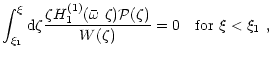
This can be seen combining Eqs. (18) and (19), and assuming as before
![]() ,
but this time leaving the
azimuthal current as a general driving term:
,
but this time leaving the
azimuthal current as a general driving term:
 |
|||
 |
(53) |
 |
(54) |
A note of caution is needed here, since the drift is actually a particle phenomenon, and needs careful handling to translate to the fluid context. However, the cold plasma model is unusual in that the linearised equations for a species fluid are identical in form to those for an individual particle, except that the electric and magnetic fields are functions of the total particle dynamics via the current and charge density equations.
Moreover, the azimuthal drift current produced by the magnetic inhomogeneity must remain bounded, in order to be consistent with the linearised modelling elsewhere.
Analytical solutions for steady small amplitude wave motion are presented in Sects. 2.1 and 2.2 for a homogeneous equilibrium plasma. (Note that the solutions in Sect. 2.2 do not describe transients.)
However for the case of an inhomogeneous magnetic field the set of Eqs. (11)-(19) although still linear does not have a closed-form analytical solution, and so we must solve the problem numerically.
The form of Eqs. (11)-(19) is suitable for
relatively straightforward numerical integration, with perturbed
velocity fields as the initial conditions (see later discussion). The
equations for
![]() and
and
![]() are
amenable to solution via a Lax-Wendroff type method, since they are
fundamentally hyperbolic in nature. The remaining equations are
ordinary differential equations, and therefore suitable for a
Runge-Kutta approach.
are
amenable to solution via a Lax-Wendroff type method, since they are
fundamentally hyperbolic in nature. The remaining equations are
ordinary differential equations, and therefore suitable for a
Runge-Kutta approach.
A vital aspect of any such numerical modelling lies in ensuring
that the ![]() drift is accounted for, in order to provide
the requisite azimuthal current density at the grid values
appropriate for the Lax-Wendroff computation. This differential
azimuthal velocity is essentially a second-order effect, and if
the system is stimulated in the electrostatic mode, it remains the
only such effect (since to first order, b-d =0). Given the
underlying symmetry, the drift is actually evaluated very close to
the grid points by the Runge-Kutta algorithm. However it is clear
that this drift must remain bounded in order to maintain
acceptable limits in accuracy between the two numerical
techniques, meaning that the magnetic gradient cannot be too
large.
drift is accounted for, in order to provide
the requisite azimuthal current density at the grid values
appropriate for the Lax-Wendroff computation. This differential
azimuthal velocity is essentially a second-order effect, and if
the system is stimulated in the electrostatic mode, it remains the
only such effect (since to first order, b-d =0). Given the
underlying symmetry, the drift is actually evaluated very close to
the grid points by the Runge-Kutta algorithm. However it is clear
that this drift must remain bounded in order to maintain
acceptable limits in accuracy between the two numerical
techniques, meaning that the magnetic gradient cannot be too
large.
At each time step it is necessary therefore to combine the Runge-Kutta and the Lax-Wendroff finite difference approaches. However it is possible to discuss the methods independently.
The next sections deal with the numerical approach.
The equations to be solved here are:
Finally, since the magnetic field gradient lies in the radial direction, we anticipate
that the drift velocity will lie in the azimuthal direction. Strictly, the updating of the
local magnetic field strength corresponding to the particle's perturbed position is a
second-order correction, and therefore is really a non-linear correction. However, the
magnetic field that appears on the right-hand side as the parameter p1 is the equilibrium
one, and its gradient is prescribed. Note that the ![]() must be significant over a
Larmor orbit, otherwise there can be no drift, and so it could be argued that the size of
this gradient makes this second-order contribution technically of a similar magnitude to the
first order ones, and certainly bigger than any
must be significant over a
Larmor orbit, otherwise there can be no drift, and so it could be argued that the size of
this gradient makes this second-order contribution technically of a similar magnitude to the
first order ones, and certainly bigger than any
![]() advective
non-linearity. Hence some preliminary justification for updating the field strength along
the particle trajectory is possible, particularly if these corrections are seen as a
quasi-linear coupling between the linear, homogeneous modes.
advective
non-linearity. Hence some preliminary justification for updating the field strength along
the particle trajectory is possible, particularly if these corrections are seen as a
quasi-linear coupling between the linear, homogeneous modes.
The standard 1-spatial dimension explicit Lax-Wendroff finite difference solver is
applied to the remaining equations, cast as a vector system:
 |
(62) |
| (63) | |
 |
(64) |
 |
(65) |
| |
= | (66) | |
| (67) |
| |
= | (68) | |
| = | (69) |
 |
(70) |
The time derivatives
![]() ,
are supplied via the R-K Eqs. (55)-(61), which are solved simultaneously with the L-W equations.
,
are supplied via the R-K Eqs. (55)-(61), which are solved simultaneously with the L-W equations.
To simplify matters, the velocity field is perturbed as the initial
condition, driving the plasma evolution. As in Paper I the
perturbations are confined to a sub-range of the full spatial
mesh: in other words, if the spatial range is [1, mm], then the
initial perturbation ranges over
![]() ,
with m2=mm/2. Moreover, in order to avoid sharp
gradients at the edges of the initial perturbation, the form of
the initial disturbance across its whole range 2mr is
multiplied by a Gaussian envelope.
,
with m2=mm/2. Moreover, in order to avoid sharp
gradients at the edges of the initial perturbation, the form of
the initial disturbance across its whole range 2mr is
multiplied by a Gaussian envelope.
The perturbation is calculated as follows:
![$\displaystyle {f(m)=\sin\left(\pi\frac{m-m_i}{m_r}\right)\exp\left[-\left(\lambda\frac{m-m_2}{m_r}\right)^2\right]}$](/articles/aa/full/2002/19/aah3345/img132.gif) |
(71) | ||
| (72) | |||
| a(mh)=a0 f(m) | (73) | ||
| q(mh)=(b0-d0) f(m) | (74) | ||
| (75) | |||
| c(mh)=c0 f(m) | (76) | ||
| d(mh)=d0 f(m). | (77) |
The values of p2 and p3 are chosen to be consistent with non-relativistic velocities as in Paper I. Moreover, all perturbation coefficients are chosen such that the results do not violate the linear nature of the calculation.
When calculating the mode coupling due to the magnetic gradient, the initial conditions here are
identical to those for the electrostatic mode, but this time the magnetic field has a
constant gradient, increasing linearly with increasing spatial mesh point. Hence the
magnetic field takes the form
| p1=p10+p11 x | (78) |
The only boundary condition at finite distance is at ![]() .
Since the region of excitation is far from the origin, two waves must propagate away from
the source region in opposite directions. There is therefore a delay before the inward propagating
wave reaches this boundary and is reflected, meaning that it is possible
to stop the calculation before such a reflection takes place, simplifying
the numerics. All the calculations reported here employ this tactic.
.
Since the region of excitation is far from the origin, two waves must propagate away from
the source region in opposite directions. There is therefore a delay before the inward propagating
wave reaches this boundary and is reflected, meaning that it is possible
to stop the calculation before such a reflection takes place, simplifying
the numerics. All the calculations reported here employ this tactic.
| mm | 500 | number of spatial points |
| n | 5000 | number of time steps |
| h | 0.7 | spatial mesh increment |
| p | 0.3 | ration spatial/temporal meshes |
| 10 | Gaussian coefficient | |
| p10 | 1.0 | magnetic field amplitude |
| p11 | 3.0 e-3 | magnetic gradient |
| p2 | 4 | mesh plasma frequency, squared |
| p3 | 1.2e-2 | normalized c2 |
| mr | 25 | half-width of initial perturbation |
Using the stated algorithms, it was possible to produce a set of numerical results, separating the normal modes from the coupling of them through the magnetic gradient. In all figures only 1% of the time steps was plotted for reasons of clarity.
The electrostatic mode, with radial electron and positron motion yielding a radial electric field, is shown in Figs. 1 and 2 for the case of a uniform magnetic field. The simulations show a confined and regular oscillation in the radial components; all other quantities are identically zero. As expected no electromagnetic wave is present.
![\begin{figure}
\par\includegraphics[width=7.5cm,clip]{rhohomr.eps} \end{figure}](/articles/aa/full/2002/19/aah3345/img143.gif) |
Figure 1: Computed radial electric field for a pure electrostatic oscillation in a uniform magnetic field. |
| Open with DEXTER | |
![\begin{figure}
\par\includegraphics[width=7.5cm,clip]{velrehomr.eps}\end{figure}](/articles/aa/full/2002/19/aah3345/img144.gif) |
Figure 2: Computed radial velocity component for electrons for a pure electrostatic oscillation in a uniform magnetic field. |
| Open with DEXTER | |
The electromagnetic mode for a uniform magnetic field might be initiated by the boundary
condition b0=0.1, d0=-0.1 applied at time ![]() over the same restricted range of
radial mesh points as the electrostatic case, with
over the same restricted range of
radial mesh points as the electrostatic case, with
![]() .
Since the
purpose of this paper is to show the connection between electrostatic and electromagnetic
modes, and since the latter do not create the former, this case will not be shown.
.
Since the
purpose of this paper is to show the connection between electrostatic and electromagnetic
modes, and since the latter do not create the former, this case will not be shown.
When a magnetic field gradient is introduced, the results are
shown in Figs. 3-10. These first results
show the persistence of the electrostatic-type behaviour, but with
a transmitted electromagnetic wave escaping from the locality of
the original disturbance. This agrees with the discussion in
Sect. 2, where it was stated that the magnetic field gradient
forces an azimuthal current in the "electrostatic'' mode via the
magnetic drift, and an electromagnetic wave is generated. In this
case given the initial conditions, and our tactic of stopping the numerical solution before
the transient wave reaches the origin (![]() ),
there are two waves propagating in opposite
directions. Note there is no contradiction with solution (52),
where the boundary condition at
),
there are two waves propagating in opposite
directions. Note there is no contradiction with solution (52),
where the boundary condition at ![]() is taken into account; the numerical
solution is simply at sufficiently early times.
is taken into account; the numerical
solution is simply at sufficiently early times.
Note that Eq. (51) suggests that the propagating wave acquires its characteristic frequency from the driving term, namely the drift current. This latter frequency is double that of the uncoupled electrostatic mode, since it is produced by the higher-order quadratic coupling inherent in q, as seen in the last two terms on the right-hand side of Eq. (57). Hence the generated electromagnetic wave automatically satisfies Eq. (50), and so is able to propagate. This is evident in Figs. 6 and 8, when compared with Fig. 4, and is presented more clearly in Fig. 10, where the temporal behaviour at a point in the centre of the oscillation is compared with that in the propagation region; the frequency in the propagation zone is nearly double that in the central oscillation.
The radiating fields obtained are very small simply because the coupling is a second-order effect, and therefore limited in magnitude for consistency. In a fully non-linear treatment this restriction does not apply.
![\begin{figure}
\par\includegraphics[width=7.5cm,clip]{velregradr.eps}\end{figure}](/articles/aa/full/2002/19/aah3345/img147.gif) |
Figure 3: Computed radial velocity component for electrons in a magnetic field gradient. |
| Open with DEXTER | |
![\begin{figure}
\par\includegraphics[width=7.5cm,clip]{rhogradr.eps}\end{figure}](/articles/aa/full/2002/19/aah3345/img148.gif) |
Figure 4: Computed radial electric field component in a magnetic field gradient. |
| Open with DEXTER | |
![\begin{figure}
\par\includegraphics[width=8.6cm,clip]{rhog550r.eps}\end{figure}](/articles/aa/full/2002/19/aah3345/img149.gif) |
Figure 5: Snapshot of evolution of radial electric field component in a magnetic field gradient, for time step 500 (solid line) and 5000 (dotted line). |
| Open with DEXTER | |
![\begin{figure}
\par\includegraphics[width=7.5cm,clip]{thegradr.eps}\end{figure}](/articles/aa/full/2002/19/aah3345/img150.gif) |
Figure 6: Computed azimuthal electric field component in a magnetic field gradient. |
| Open with DEXTER | |
![\begin{figure}
\par\includegraphics[width=8.6cm,clip]{theg550r.eps}\end{figure}](/articles/aa/full/2002/19/aah3345/img151.gif) |
Figure 7: Snapshot of evolution of azimuthal electric field component in a magnetic field gradient, for time step 500 (solid line) and 5000 (dotted line). |
| Open with DEXTER | |
![\begin{figure}
\par\includegraphics[width=7.5cm,clip]{betgradr.eps}\end{figure}](/articles/aa/full/2002/19/aah3345/img152.gif) |
Figure 8: Computed perturbed axial magnetic field component, in a magnetic field gradient. |
| Open with DEXTER | |
![\begin{figure}
\par\includegraphics[width=8.6cm,clip]{betg550r.eps}\end{figure}](/articles/aa/full/2002/19/aah3345/img153.gif) |
Figure 9: Snapshot of evolution of axial magnetic field component in a magnetic field gradient, for time step 500 (solid line) and 5000 (dotted line). |
| Open with DEXTER | |
![\begin{figure}
\par\includegraphics[width=8.6cm,clip]{rhother.eps}\end{figure}](/articles/aa/full/2002/19/aah3345/img154.gif) |
Figure 10: Comparison of the time evolution of the radial electric field at the centre point of the initial disturbance (solid line, left-hand axis) with the azimuthal electric field at a point in the propagation zone (dotted line, right-hand axis). Note the frequency doubling in the latter, due to the higher-order drift current interaction. |
| Open with DEXTER | |
This paper shows that provided a cold e-p magnetoplasma has an inhomogeneous magnetic field, which are conditions present in pulsar magnetospheres and in particular the magnetospheric plasma rest frame, any electrostatic perturbation will be able to generate an electromagnetic wave propagating away in all directions by virtue of the drift currents. This was demonstrated in the context of a linear approximation, but we expect that a general full non-linear calculation will confirm these findings. Moreover, this mechanism will undoubtedly play a significant part in quenching the density instability found in Paper I, by radiating away the total energy content of the large amplitude oscillation before the onset of the large velocities that are characteristic of unstable density evolution. However, given that this linearised calculation is necessarily limited in the radiation amplitude that it can generate, only a full non-linear calculation show instability quenching in this way.
In fact, the full, non-linear evolution of the plasma will automatically produce large inhomogeneities in all the fields, so that there is the possibility that even with an initially homogeneous magnetic field, electromagnetic radiation might still be created. This simulation is currently underway, and will be reported here soon.
It is appropriate also to note that in the cold, fluid context the existence of a strong magnetic field gradient will mean that the equilibrium density distribution of particles in practice will not be uniform, since the plasma will tend to avoid regions of strong magnetic pressure; however, the equilibrium density is assumed constant here, though the numerical algorithms can be extended to incorporate the effect.
Finally, it is expected that in a pulsar magnetosphere these plasma rest frame phenomena will assume great significance in the laboratory frame as stated in Paper I. Since we might still expect the quasi-static condition to hold, and therefore this mechanism to rotate around with the angular velocity of the pulsar, the radiated frequency in the rest frame has to be Doppler shifted to the laboratory frame taking into account the Lorentz factor of the moving plasma. The linear calculation shows frequency doubling arising from the drift current; a full non-linear calculation will yield a characteristic spectrum of frequencies reflecting local ambient plasma conditions at the oscillation site. If a broad space region is implicated in such radiating oscillations, then it seems clear that the resulting radiation will be broadband even in the plasma rest frame. If this source is rotating outside the speed of light cylinder (da Costa & Kahn 1985), radiation generation in the rest frame might be the basis for a real superluminal lighthouse effect.
Acknowledgements
The present work was developed in two visits, one (DAD) to Lisbon, May 2001, supported by both Centro de Electrodinâmica, and the Astronomy & Astrophysics Group of Department of Physics and Astronomy, University of Glasgow; the other (AAC) to Glasgow, October 2001 supported by the PPARC Short Term Visitors Grant PPA/V/S/2000/00572.