A&A 386, 732-742 (2002)
DOI: 10.1051/0004-6361:20020306
Gravitational instability of polytropic spheres and generalized thermodynamics
P. H. Chavanis
Laboratoire de Physique Quantique, Université Paul Sabatier, 118
route de Narbonne 31062 Toulouse, France
Institute for
Theoretical Physics, University of California, Santa Barbara,
California CA93106, USA
Received 18 September 2001 / Accepted 30 January 2002
Abstract
We extend the existing literature on the structure and
stability of polytropic gas spheres reported in the classical
monograph of Chandrasekhar (1932). For isolated polytropes with
index 1<n<5, we provide a new, alternative, proof that the onset
of gravitational instability occurs for n=3 and we express the
perturbation profiles of density and velocity at the point of
marginal stability in terms of the Milne variables. Then, we
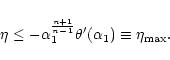
consider the case of polytropes confined within a box of radius R (an extension of the Antonov problem for isothermal gas
spheres). For  ,
the mass-density relation presents damped
oscillations and there exists a limiting mass above which no
hydrostatic equilibrium is possible. As for isothermal gas
spheres, the onset of instability occurs precisely at the point of
maximum mass in the series of equilibrium. Analytical results are
obtained for the particular index n=5. We also discuss the
relation of our study with generalized thermodynamics (Tsallis
entropy) recently investigated by Taruya & Sakagami
(2002).
,
the mass-density relation presents damped
oscillations and there exists a limiting mass above which no
hydrostatic equilibrium is possible. As for isothermal gas
spheres, the onset of instability occurs precisely at the point of
maximum mass in the series of equilibrium. Analytical results are
obtained for the particular index n=5. We also discuss the
relation of our study with generalized thermodynamics (Tsallis
entropy) recently investigated by Taruya & Sakagami
(2002).
Key words: hydrodynamics - instabilities - stars: oscillations
1 Introduction
In earlier papers of this series (Chavanis 2002a,b,c) we investigated
the gravitational instability of finite isothermal spheres in
Newtonian gravity and general relativity for classical particles and
for quantum particles (fermions). From a theoretical point of view,
these systems exhibit interesting behavior with the occurence of
phase transitions associated with gravitational collapse (Antonov
1962; Lynden-Bell & Wood 1968; Padmanabhan 1990). A rich stability
analysis follows and can be conducted analytically or by using
graphical constructions. From an astrophysical point of view, these
studies can be relevant for various systems, including elliptical
galaxies, globular clusters, the interstellar medium, the core of
neutron stars and dark matter made of massive neutrinos.
In this paper, we propose to extend our study to the case of
polytropic gas spheres. Polytropes with index 1<n<5 are
self-confined, so it is not necessary to introduce an artificial
``box'' to limit their spatial extent. Using the methods developed
for isothermal configurations, we show that the transition from
stability to instability corresponds to an index n=3. This result is
well-known but we provide a new derivation based on the exact
resolution of the pulsation equation for polytropes. The perturbation
profiles at the point of marginal stability are expressed in terms of
the Milne variables (Chandrasekhar 1932). The profile of density
perturbation has only one node and the velocity perturbation is
proportional to the radial distance.
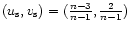
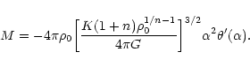
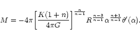
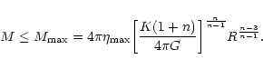
Then, we consider the case of polytropes with arbitrary index n>1confined within a box of radius R. For  ,
we recover the
classical Antonov (1962) problem for isothermal gas spheres. However,
for
we already obtain results strikingly similar to those
obtained for isothermal configurations. In particular, confined
polytropes in hydrostatic equilibrium can exist only below a limiting
mass (for a given box radius R) and the series of equilibrium
becomes unstable precisely at the point of maximum mass. Subsequent
oscillations in the mass-density profile (for n>5) are associated
with secondary modes of instability. The locii of these modes of
instability follow a geometric progression with a ratio depending on
the index of the polytrope. For ,
we recover the ratio
10.74... of isothermal gas spheres.
,
we recover the
classical Antonov (1962) problem for isothermal gas spheres. However,
for
we already obtain results strikingly similar to those
obtained for isothermal configurations. In particular, confined
polytropes in hydrostatic equilibrium can exist only below a limiting
mass (for a given box radius R) and the series of equilibrium
becomes unstable precisely at the point of maximum mass. Subsequent
oscillations in the mass-density profile (for n>5) are associated
with secondary modes of instability. The locii of these modes of
instability follow a geometric progression with a ratio depending on
the index of the polytrope. For ,
we recover the ratio
10.74... of isothermal gas spheres.
While this paper was in preparation, we came across the preprint of
Taruya & Sakagami (2002) on a related subject. These authors
investigate the stability of polytropes in the framework of extended
thermodynamics, using Tsallis entropy. Therefore, in Sect.
4, we analyze the connexion of the present study with
their approach and we discuss the relevance of Tsallis entropy for
describing astrophysical systems.
2 Properties of polytropic gas spheres
2.1 The Lane-Emden equation
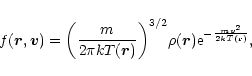
Polytropic stars are characterized by an equation of state of the form
 |
(1) |
where K and  are constants. The index n of the polytrope is defined by the relation
 |
(2) |
The equation of state (1) corresponds to an adiabatic equilibrium in regions where convection keeps the star stirred up and produces a uniform entropy distribution (
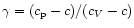
 ). In that case,
is the ratio of specific heats
cp/cV at constant pressure and volume. For a monoatomic gas,
). In that case,
is the ratio of specific heats
cp/cV at constant pressure and volume. For a monoatomic gas,
 .
The equation of state (1) also describes a polytropic equilibrium characterized by a uniform specific heat
.
The equation of state (1) also describes a polytropic equilibrium characterized by a uniform specific heat
 .
In this more general situation
.
In this more general situation
 .
Convective equilibrium is recovered for c=0 and isothermal equilibrium is obtained in the limit of infinite specific heat
.
Convective equilibrium is recovered for c=0 and isothermal equilibrium is obtained in the limit of infinite specific heat
 .
A power law relation between the pressure and the density is also the limiting form of the equation of state describing a gas of cold degenerate fermions (Chandrasekhar 1932). In that case, the constant K can be expressed in terms of fundamental constants. In the classical limit
,
n=3/2 and
.
A power law relation between the pressure and the density is also the limiting form of the equation of state describing a gas of cold degenerate fermions (Chandrasekhar 1932). In that case, the constant K can be expressed in terms of fundamental constants. In the classical limit
,
n=3/2 and
 (where h is the Planck constant) and in the relativistic limit
 ,
n=3 and
,
n=3 and
 (where c is the speed of light). Historically, the index
appears in the classical theory of white dwarf stars initiated by Fowler (1926) and the index
is related to the limiting mass of Chandrasekhar (1931).
(where c is the speed of light). Historically, the index
appears in the classical theory of white dwarf stars initiated by Fowler (1926) and the index
is related to the limiting mass of Chandrasekhar (1931).
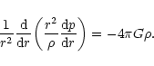
The condition of hydrostatic equilibrium for a spherically symmetrical distribution of matter reads
 |
(3) |
where  is the gravitational potential. Using the Gauss theorem
 |
(4) |
where
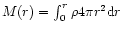 is the mass contained within the sphere of radius r, we can derive the fundamental equation of equilibrium (Chandrasekhar 1932)
 |
(5) |
Equations (1), (5) fully determine the structure of polytropic gas spheres. Letting
 |
(6) |
where  is the central density, we can reduce the condition of hydrostatic equilibrium to the Lane-Emden equation (Chandrasekhar 1932)
 |
(7) |
with boundary conditions
 |
(8) |
For n>3, the Lane-Emden equation admits an analytical solution which is singular at the origin:
 |
(9) |
Regular solutions of the Lane-Emden equation must in general be computed numerically. For
 ,
we can expand the function
,
we can expand the function  in Taylor series. The first terms in this expansion are given by
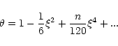 |
(10) |
The behavior of
 at large distances deserves a more
specific discussion. For 1<n<5, the density falls off to zero at a
finite radius R, identified as the radius of the star. If we denote
by
at large distances deserves a more
specific discussion. For 1<n<5, the density falls off to zero at a
finite radius R, identified as the radius of the star. If we denote
by  the value of the normalized distance at which
  then, for
 ,
we have
,
we have
 |
(11) |
For n>5, the polytropes extend to infinity, like the isothermal configurations recovered in the limit .
For
 ,
,
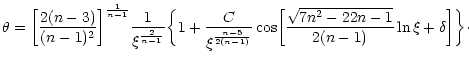 |
|
|
(12) |
The curve (12) intersects the singular solution (9)
infinitely often at points that asymptotically increase geometrically
in the ratio 1:
 .
Since
.
Since
 at large distances, these
configurations have an "infinite mass'', which is clearly
unphysical. In the following, we shall restrict these configurations to a
"box'' of radius R, as in the classical Antonov
problem. Therefore, Eq. (7) must be solved for
at large distances, these
configurations have an "infinite mass'', which is clearly
unphysical. In the following, we shall restrict these configurations to a
"box'' of radius R, as in the classical Antonov
problem. Therefore, Eq. (7) must be solved for
 with
with
 |
(13) |
Note that, for a fixed box radius R,  is a measure of the central density .
The case n=5 is special. For this index, the Lane-Emden equation can be solved analytically and yields the result:
is a measure of the central density .
The case n=5 is special. For this index, the Lane-Emden equation can be solved analytically and yields the result:
 |
(14) |
The total mass of this configuration is finite but its potential energy diverges. Therefore, this polytrope must also be confined within a box. In Fig. 1, we have plotted different density profiles with index n=3,5,6.
![\begin{figure}
\par\includegraphics[width=8.8cm,clip]{profilesP.eps}\end{figure}](/articles/aa/full/2002/17/aa1920/Timg40.gif) |
Figure 1:
Density profiles of polytropes with index n=3,5,6. The dashed line corresponds to the singular solution (9). |
| Open with DEXTER |
2.2 The Milne variables
As in the analysis of isothermal gas spheres, it will be convenient in the following to introduce the Milne variables (u,v) defined by (Chandrasekhar 1932):
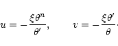 |
(15) |
Taking the logarithmic derivative of u and v with respect to  and using Eq. (7), we get
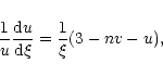 |
(16) |
 |
(17) |
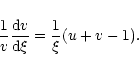
Due to the homology invariance of the polytropic configuations (see Chandrasekhar 1932), the Milne variables u and v satisfy a first order differential equation
 |
(18) |
The solution curve in the (u,v) plane (see Figs. 2-4) is parametrized by .
It starts from the point
(u,v)=(3,0) with a slope
 as
.
For 1<n<5, the curve is monotonous and tends to
as
.
For 1<n<5, the curve is monotonous and tends to
 as
.
More precisely, using Eq. (11), we have
as
.
More precisely, using Eq. (11), we have
 |
(19) |
For n>5, the solution curve spirals indefinitely around the fixed point
 ,
corresponding to the singular solution (9), as
tends to infinity. All polytropic spheres must necessarily lie on this curve. For bounded polytropic spheres,
must be terminated at the box radius .
For n=5, the Milne variables are related according to
,
corresponding to the singular solution (9), as
tends to infinity. All polytropic spheres must necessarily lie on this curve. For bounded polytropic spheres,
must be terminated at the box radius .
For n=5, the Milne variables are related according to
![\begin{figure}
\par\includegraphics[width=8.8cm,clip]{uv4P.eps}\end{figure}](/articles/aa/full/2002/17/aa1920/Timg50.gif) |
Figure 2:
The (u,v) plane for polytropes with index 1<n<5. The construction is made explicitly for n=4. |
| Open with DEXTER |
![\begin{figure}
\par\includegraphics[width=8.8cm,clip]{uv6P.eps}\end{figure}](/articles/aa/full/2002/17/aa1920/Timg52.gif) |
Figure 4:
The (u,v) plane for polytropes with index n>5. The construction is made explicitly for n=6. |
| Open with DEXTER |
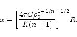
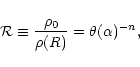
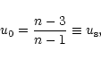
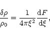
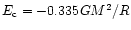
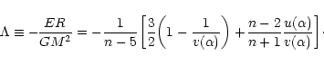
2.3 The maximum mass and minimum temperature of confined polytropes
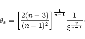
For polytropes confined within a box of radius R, there exists a well-defined relation between the mass M of the configuration and the central density
(through the parameter ). Starting from the relation
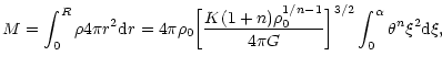 |
|
|
(21) |
and using the Lane-Emden Eq. (7), we get
 |
(22) |
Expressing the central density in terms of ,
using Eq. (13), we obtain after some rearrangements
 |
(23) |
Introducing the parameter
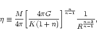 |
(24) |
the foregoing relation can be rewritten
 |
(25) |
For n<5, the normalized box radius
in necessarily
restricted by the inequality
 .
For the limiting
value
.
For the limiting
value
 ,
corresponding to an isolated polytrope satisfying
,
corresponding to an isolated polytrope satisfying
 ,
we have
,
we have
 |
(26) |
The quantity
 ,
defined by Eq. (19), has been tabulated by
Chandrasekhar (1932). The definition (24) of
,
defined by Eq. (19), has been tabulated by
Chandrasekhar (1932). The definition (24) of  and the
relation (25) between
and
are consistent with
the formulae derived in the case of an isothermal gas (see
Chavanis 2002a). This connexion is particularly relevant if we interpret
the constant K as a polytropic temperature
and the
relation (25) between
and
are consistent with
the formulae derived in the case of an isothermal gas (see
Chavanis 2002a). This connexion is particularly relevant if we interpret
the constant K as a polytropic temperature
 (see
Chandrasekhar 1932, p. 86). For
(see
Chandrasekhar 1932, p. 86). For
 ,
,
 and the parameter
reduces to the corresponding one for isothermal spheres
(
and the parameter
reduces to the corresponding one for isothermal spheres
(
 ,
,
 ,
,
 ).
).
![\begin{figure}\par\includegraphics[width=8.8cm]{alphaetaP.eps}\end{figure}](/articles/aa/full/2002/17/aa1920/Timg70.gif) |
Figure 5:
Mass-density profiles for polytropic configurations with index
n=2,3,4,5,6. A mass peak appears for the first time for the critical index n=3. |
| Open with DEXTER |
The function
 is represented in Fig. 5 for
different values of the polytropic index n. Instead of ,
we could have used the density contrast
is represented in Fig. 5 for
different values of the polytropic index n. Instead of ,
we could have used the density contrast
 |
(27) |
which also provides a relevant parametrization of the solutions.
Using the Lane-Emden Eq. (7) and the definition of the
Milne variables (15), it is straightforward to check that the
condition of extremum
 is equivalent to
 |
(28) |
where, by definition,
 and
and
 refers to the singular solution (9). For
 ,
we recover the condition u0=1 previously derived for isothermal configurations (Chavanis 2002a). The values of
for which
is extremum are given by the intersection(s) between the solution curve in the (u,v) plane and the line u=us (see Figs. 2-4). For 1<n<3,
,
we recover the condition u0=1 previously derived for isothermal configurations (Chavanis 2002a). The values of
for which
is extremum are given by the intersection(s) between the solution curve in the (u,v) plane and the line u=us (see Figs. 2-4). For 1<n<3,
 and there is no intersection. The mass-density relation is therefore monotonous. For
 ,
the curve
presents a single maximum at
,
the curve
presents a single maximum at
 .
For n=3, this maximum is reached at the extremity of the curve (
.
For n=3, this maximum is reached at the extremity of the curve (
 ). For n=5,
 and the function
is explicitly given by
and the function
is explicitly given by
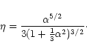 |
(29) |
The maximum of
is located at
 .
Finally, for n>5, the mass-density relation presents an infinite number of damped oscillations since the line defined by Eq. (28) passes through the center of the spiral in the (u,v) plane. If we denote by
.
Finally, for n>5, the mass-density relation presents an infinite number of damped oscillations since the line defined by Eq. (28) passes through the center of the spiral in the (u,v) plane. If we denote by
 the locii of the extrema of
,
these values asymptotically follow the geometric
progression
the locii of the extrema of
,
these values asymptotically follow the geometric
progression
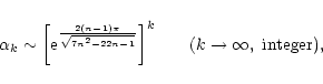 |
(30) |
obtained by substituting the asymptotic expansion (12) in Eq. (28). For
,
we recover the ratio
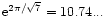 corresponding to classical isothermal configurations (Semelin et al. 1999; Chavanis 2002a).
From the above results, it is clear that restricted polytropic spheres with index
can exist only for
 |
(31) |
This implies in particular the existence of a limiting mass (for a given confining radius R) such that
 |
(32) |
For ,
we recover the limiting mass
 above which an isothermal sphere cannot sustain self-gravity (see, e.g., Chavanis 2002b). Alternatively, for a given mass M and radius R, the inequality (31) implies the existence of a minimum value of the polytropic temperature
 .
Indeed,
is restricted by the inequality
.
Indeed,
is restricted by the inequality
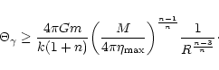 |
(33) |
In the limit ,
we recover the critical temperature
 below which an isothermal sphere is expected to collapse (Lynden-Bell & Wood 1968). This critical point, corresponding to
,
appears for the first time for the index n=3. This observation will take a deeper physical significance in the stability analysis performed in the following section. For
below which an isothermal sphere is expected to collapse (Lynden-Bell & Wood 1968). This critical point, corresponding to
,
appears for the first time for the index n=3. This observation will take a deeper physical significance in the stability analysis performed in the following section. For  ,
the mass-density profile is monotonous and
,
the mass-density profile is monotonous and
 .
The total mass (resp. temperature) of confined polytropes is always smaller (resp. larger) than the corresponding one for isolated polytropes. However, this bound does not correspond to a condition of extremum
but rather to the impossibility of constructing polytropes with
.
The total mass (resp. temperature) of confined polytropes is always smaller (resp. larger) than the corresponding one for isolated polytropes. However, this bound does not correspond to a condition of extremum
but rather to the impossibility of constructing polytropes with
 (since
can become negative).
(since
can become negative).
3 Dynamical stability of polytropic gas spheres
3.1 The equation of radial pulsations
We shall now investigate the dynamical stability of polytropic gas spheres against radial perturbations. We use a method and presentation similar to that adopted for isothermal spheres in Chavanis (2002a). The equations describing the motions of a gaseous star are the equation of continuity, the Euler equation and the Poisson equation
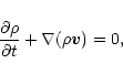 |
(34) |
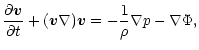 |
|
|
(35) |
 |
(36) |
It is possible to show that viscosity does not change the onset of instability. Therefore, for simplicity, we have directly used the Euler equation instead of the Navier-Stokes equation. We assume furthermore that the pressure and the density are related to each other by the polytropic equation of state (1). We write small perturbations around equilibrium in the form
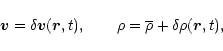 |
(37) |
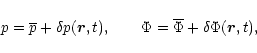 |
(38) |
where the bar refers to the stationary solution (in the following we shall drop the bar). The linearized equations for the perturbations are
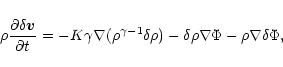 |
(39) |
 |
(40) |
 |
(41) |
Restricting ourselves to radial perturbations and writing the time dependance of
the perturbation in the form
 ,
,
 ,..., the equations of the problem become
 |
(42) |
 |
(43) |
 |
(44) |
We introduce the function q(r) by the relation
 |
(45) |
Physically, q(r) represents the mass perturbation
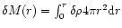 within the sphere of radius r. Thus, by definition, q(0)=0. Then, it is readily seen that the Poisson equation (44) is equivalent to
 |
(46) |
which is just the perturbed Gauss theorem (4). On the other hand, the continuity Eq. (43) leads to the relation
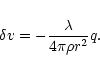 |
(47) |
Substituting these results back into Eq. (42), we obtain
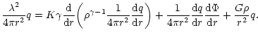 |
|
|
(48) |
Using the condition of hydrostatic equilibrium (3), the foregoing equation can be rewritten
 |
(49) |
which is the required equation of radial pulsations for a polytrope.
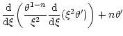
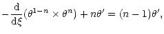
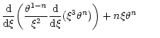
3.2 The condition of marginal stability
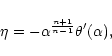
Considering the case of marginal stability  and introducing the dimensionless variables defined in Sect. 2, we can reduce the equation of radial pulsations to the form
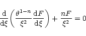 |
(50) |
with F(0)=0. Denoting by  the differential operator appearing in Eq. (50) and using the Lane-Emden Eq. (7), we easily establish that
Therefore, the general solution of Eq. (50) is
 |
(53) |
where c1 is an arbitrary constant. The connexion with isothermal configurations (see Chavanis 2002a) is particularly obvious if we make the correspondance
 and
and
 .
.
3.3 Boundary conditions
The equation of pulsations (49) must be supplemented by appropriate boundary conditions. For self-confined polytropes (1<n<5), we require that the Lagrangian derivative of the pressure vanishes at the surface of the configuration, i.e.
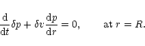 |
(54) |
Using Eqs. (45), (47), this condition can be rewritten
 |
(55) |
or, in dimensionless form,
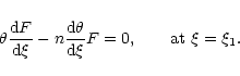 |
(56) |
The index of the marginally stable polytrope is obtained by substituting the solution (53) in the boundary condition (56). Since
 ,
this yields n=3. Therefore, the transition from stability to instability occurs for a polytropic index n=3 or, equivalently, for an adiabatic index
.
Of course, this result is well-known and could have been obtained from the general theorems of stellar pulsation (see, e.g., Cox 1980). However, we provide here an alternative method based on the explicit resolution of the equation of pulsations for polytropes.
,
this yields n=3. Therefore, the transition from stability to instability occurs for a polytropic index n=3 or, equivalently, for an adiabatic index
.
Of course, this result is well-known and could have been obtained from the general theorems of stellar pulsation (see, e.g., Cox 1980). However, we provide here an alternative method based on the explicit resolution of the equation of pulsations for polytropes.
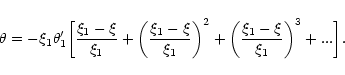
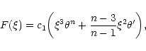
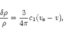
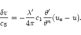
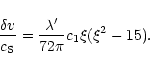
According to Eq. (45), the perturbation profile at the point of marginal stability is given by
 |
(57) |
with the expression (53) for  .
Simplifying the derivative with the aid of the Lane-Emden Eq. (7), we obtain
.
Simplifying the derivative with the aid of the Lane-Emden Eq. (7), we obtain
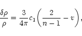 |
(58) |
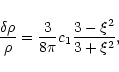
where v is the Milne variable (15). For n=3, it reduces to
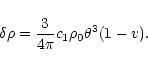 |
(59) |
This perturbation profile is plotted in Fig. 6. It has one node
at
 On the other hand, the velocity profile is
given by Eq. (47). Normalizing with a typical velocity
On the other hand, the velocity profile is
given by Eq. (47). Normalizing with a typical velocity
 ,
we find that
,
we find that
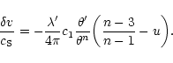 |
(60) |
We assume that we are just at the onset of the instability
 so that Eq. (60) is applicable with
 .
Substituting explicitly for n=3, we get
.
Substituting explicitly for n=3, we get
 |
(61) |
and we observe that the velocity is proportional to the radial distance (see also Cox 1980).
![\begin{figure}
\par\includegraphics[width=8.8cm,clip]{deltarho3P.eps}\end{figure}](/articles/aa/full/2002/17/aa1920/Timg142.gif) |
Figure 6:
Density perturbation profile for the critical polytrope of index
n=3. |
| Open with DEXTER |
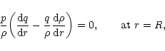
For polytropes confined within a box, the boundary condition consistent with the conservation of mass is
 .
With the expression (53) for ,
this yields
.
With the expression (53) for ,
this yields
 |
(62) |
which is precisely Eq. (28). Therefore, the point of marginal stability coincides with the point of maximum mass (or minimum temperature) in the series of equilibrium. For n<3, restricted polytropes are always stable since the function
is monotonous. For
,
the configurations with
 are unstable but there are no secondary instabilities. For n>5, a first mode of stability is lost for
 .
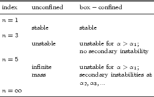
Subsequent oscillations in the mass-density profile are associated with secondary instabilities. A summary of the stability limits for polytropic gas spheres is given in Table 1. In Fig. 7 we have plotted the density contrast at the critical point
as a function of the index of the polytrope. For ,
the polytropes are stable and
.
Subsequent oscillations in the mass-density profile are associated with secondary instabilities. A summary of the stability limits for polytropic gas spheres is given in Table 1. In Fig. 7 we have plotted the density contrast at the critical point
as a function of the index of the polytrope. For ,
the polytropes are stable and
 .
For n>3, only configurations with a density contrast
.
For n>3, only configurations with a density contrast
 are stable. For
,
the critical density contrast tends to its classical value
are stable. For
,
the critical density contrast tends to its classical value
 (see Chavanis 2002a).
![\begin{figure}
\par\includegraphics[width=8.8cm,clip]{ncontrastP.eps}\end{figure}](/articles/aa/full/2002/17/aa1920/Timg150.gif) |
Figure 7:
Critical density contrast as a function of the polytropic
index n. |
| Open with DEXTER |
Using Eqs. (58), (60), the profiles of density and velocity that trigger the instabilities at the critical points can be written
 |
(63) |
 |
(64) |
where we recall that
 for the mode of instability of order k. We can determine the qualitative behavior of these profiles graphically by considering the intersections between the solution curve in the (u,v) plane and the lines
 and
and
 (see Figs. 2-4). These intersections determine the nodes of the perturbation profile. For
,
there is only one intersection since the (u,v) curve is monotonous. For n=5, we obtain the analytical solutions
(see Figs. 2-4). These intersections determine the nodes of the perturbation profile. For
,
there is only one intersection since the (u,v) curve is monotonous. For n=5, we obtain the analytical solutions
 |
(65) |
 |
(66) |
The perturbation
 has its node at
 .
For n>5, there are several intersections with the spiral since the lines
and
pass through the fixed point. The description of the perturbation profiles is similar to the one given for isothermal spheres (). The density profile of the fundamental mode of instability (at
)
has only one node. High order modes of instability (at
.
For n>5, there are several intersections with the spiral since the lines
and
pass through the fixed point. The description of the perturbation profiles is similar to the one given for isothermal spheres (). The density profile of the fundamental mode of instability (at
)
has only one node. High order modes of instability (at
 ,
k>1) present numerous oscillations whose nodes asymptotically follow a geometric progression. We refer to our previous paper (Chavanis 2002a) for a more precise description of these results.
,
k>1) present numerous oscillations whose nodes asymptotically follow a geometric progression. We refer to our previous paper (Chavanis 2002a) for a more precise description of these results.
Table 1:
Summary of the stability limits for polytropic gas spheres.
 |
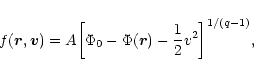
4 Generalized thermodynamics and Tsallis entropy
Recently, Taruya & Sakagami (2002) have investigated the stability of polytropic spheres within the framework of generalized thermodynamics. It has been argued by Tsallis and co-workers that ordinary statistical mechanics and thermodynamics does not describe correctly systems with long-range interactions, which are in essence non extensive. A family of functionals of the form
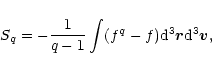 |
(67) |
known as Tsallis entropies, has been introduced to extend the classical Boltzmann-Gibbs statistical mechanics to these systems. These functionals are labeled by a parameter q. The Boltzmann entropy is recovered in the limit
 .
This new formalism has been applied in various domains of physics, astrophysics, fluid mechanics, biology, economy etc. and it extends the results obtained with ordinary statistical mechanics. In the case of self-gravitating systems, it was shown by Plastino & Plastino (1993) that the extremalization of the Tsallis entropy at fixed mass and energy yields a polytropic equation of state of the form (1). The parameter q is related to the index n of the polytrope by the relation
.
This new formalism has been applied in various domains of physics, astrophysics, fluid mechanics, biology, economy etc. and it extends the results obtained with ordinary statistical mechanics. In the case of self-gravitating systems, it was shown by Plastino & Plastino (1993) that the extremalization of the Tsallis entropy at fixed mass and energy yields a polytropic equation of state of the form (1). The parameter q is related to the index n of the polytrope by the relation
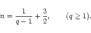 |
(68) |
Then, Taruya & Sakagami (2002) investigated the stability problem in
the microcanonical ensemble by extending the analysis of Padmanabhan
(1989) for the classical Antonov instability. Polytropic
configurations are said to be stable if they correspond to
(generalized) entropy maxima at fixed mass M and energy E.
Taruya & Sakagami showed that, for n>5, an equilibrium exists only
above a critical energy
 depending on the index of the
configuration. In the limit
,
the Antonov result
depending on the index of the
configuration. In the limit
,
the Antonov result
 obtained with the Boltzmann entropy is
recovered. Furthermore, they showed that the onset of instability
coincides with the point of minimum energy in the series of
equilibrium in agreement with standard turning point analysis (e.g.,
Katz 1978). For n<5, there is no critical value of energy and the
polytropic configurations are stable. These results differ from those
obtained in the present paper where it is found that the index marking
the transition from stability to instability is n=3 (in agreement
with standard theorems of stellar pulsations). The origin of this
discrepency is certainly related to the inequivalence of statistical
ensembles in extended thermodynamics, like in ordinary thermodynamics,
for self-gravitating systems (see, e.g., Padmanabhan 1990; Chavanis
2002c; Chavanis et al. 2002). Taruya & Sakagami work in the
microcanonical ensemble and maximize Tsallis entropy at fixed mass and
energy. On the contrary, in our study, we keep the polytropic
temperature
constant, which corresponds to the
canonical description. It would be of interest to study the
maximization of Tsallis free energy at fixed mass and temperature to
see if it provides the same conditions of stability as our dynamical
approach based on the Navier-Stokes equations. For the Boltzmann
entropy, a clear connexion was found between dynamical stability and
thermodynamical stability in the canonical ensemble (Semelin et al. 2001; Chavanis 2002a) and it is desirable to check whether this
connexion is preserved by Tsallis generalized thermodynamics. This
requires in particular to define properly the notion of temperature
and free energy in the generalized sense.
obtained with the Boltzmann entropy is
recovered. Furthermore, they showed that the onset of instability
coincides with the point of minimum energy in the series of
equilibrium in agreement with standard turning point analysis (e.g.,
Katz 1978). For n<5, there is no critical value of energy and the
polytropic configurations are stable. These results differ from those
obtained in the present paper where it is found that the index marking
the transition from stability to instability is n=3 (in agreement
with standard theorems of stellar pulsations). The origin of this
discrepency is certainly related to the inequivalence of statistical
ensembles in extended thermodynamics, like in ordinary thermodynamics,
for self-gravitating systems (see, e.g., Padmanabhan 1990; Chavanis
2002c; Chavanis et al. 2002). Taruya & Sakagami work in the
microcanonical ensemble and maximize Tsallis entropy at fixed mass and
energy. On the contrary, in our study, we keep the polytropic
temperature
constant, which corresponds to the
canonical description. It would be of interest to study the
maximization of Tsallis free energy at fixed mass and temperature to
see if it provides the same conditions of stability as our dynamical
approach based on the Navier-Stokes equations. For the Boltzmann
entropy, a clear connexion was found between dynamical stability and
thermodynamical stability in the canonical ensemble (Semelin et al. 2001; Chavanis 2002a) and it is desirable to check whether this
connexion is preserved by Tsallis generalized thermodynamics. This
requires in particular to define properly the notion of temperature
and free energy in the generalized sense.
In Figs. 8-11, we have represented the equilibrium
phase diagram (for different values of n) obtained in the framework
of extended thermodynamics, interpreting the parameter
as a generalized
inverse temperature. The temperature-energy curve is defined
in a parametric form by the equations
 |
(69) |
 |
(70) |
The expression (70) for the energy has been derived by Taruya & Sakagami (2002). For n<3, there is no turning point in the diagram, so the polytropes are always stable. For 3<n<5, the inverse temperature
presents a maximum but not the energy. Therefore, the polytropes are always stable in the microcanonical ensemble but they are unstable in the canonical ensemble after the turning point. It can be noted that the unstable region has a negative specific heat
 (in the generalized sense). For n>5, the temperature and the energy both present an infinite number of extrema. For
  ,
there are crossing points at which two solutions have the same value of temperature and energy but a different density contrast (to our knowledge, this is the first time such a situation is reported). The polytropes are unstable in the canonical ensemble after the first turning point of temperature and they are unstable in the microcanonical ensemble after the first turning point of energy. These results are strikingly similar to those obtained with the classical Boltzmann entropy
,
there are crossing points at which two solutions have the same value of temperature and energy but a different density contrast (to our knowledge, this is the first time such a situation is reported). The polytropes are unstable in the canonical ensemble after the first turning point of temperature and they are unstable in the microcanonical ensemble after the first turning point of energy. These results are strikingly similar to those obtained with the classical Boltzmann entropy
 .
.
It is interesting that the results obtained for isothermal gas spheres
described by ordinary thermodynamics (Boltzmann entropy) can be
extended to polytropic configurations by introducing a generalized
functional (Tsallis entropy). This makes this new formalism of
interest. However, we would like to make two comments. (i) First of all,
Tsallis entropy does not describe polytropic gaseous stars
although it yields an equation of state of the polytropic form. Indeed,
Tsallis entropy predicts in addition a distribution function of
the form
 |
(71) |
whereas in polytropic stars, the distribution function corresponds to a local thermodynamical equilibrium (L.T.E) characterized by a Maxwellian distribution of velocities
 |
(72) |
with a local temperature
 (recall that, for convective
equilibrium, the entropy is uniform not the temperature). In view of
these remarks, the connexion between generalized thermodynamical
stability (in the canonical ensemble) and dynamical stability with
respect to Navier-Stokes equations is not obvious. It is however
expected to be true since the condition of dynamical stability is
consistent with the turning point argument of thermodynamical
stability. (ii) Tsallis entropy could describe a particular class of
stellar systems, apparently not observed in nature, known as stellar
polytropes (see Binney & Tremaine 1987). These systems have the same
structure as polytropic gas spheres in physical space but not in phase
space (the equivalence only occurs for a polytropic index ,
i.e. for an isothermal configuration). This distinction is important
because isolated stellar polytropes are always stable with respect to
the Vlasov (or collisionless Boltzmann) equation (see Binney &
Tremaine 1987) while isolated polytropic stars are unstable with
respect to the Navier-Stokes equations for .
Generalized
thermodynamics could be developed (at least formally) for this particular
class of stellar systems.
(recall that, for convective
equilibrium, the entropy is uniform not the temperature). In view of
these remarks, the connexion between generalized thermodynamical
stability (in the canonical ensemble) and dynamical stability with
respect to Navier-Stokes equations is not obvious. It is however
expected to be true since the condition of dynamical stability is
consistent with the turning point argument of thermodynamical
stability. (ii) Tsallis entropy could describe a particular class of
stellar systems, apparently not observed in nature, known as stellar
polytropes (see Binney & Tremaine 1987). These systems have the same
structure as polytropic gas spheres in physical space but not in phase
space (the equivalence only occurs for a polytropic index ,
i.e. for an isothermal configuration). This distinction is important
because isolated stellar polytropes are always stable with respect to
the Vlasov (or collisionless Boltzmann) equation (see Binney &
Tremaine 1987) while isolated polytropic stars are unstable with
respect to the Navier-Stokes equations for .
Generalized
thermodynamics could be developed (at least formally) for this particular
class of stellar systems.
However, generalized thermodynamics is often presented as a way of
solving the "problems'' associated with the use of the Boltzmann
entropy in systems with long-range interactions and we would like to
criticize this interpretation. For self-gravitating systems, the
"problems'' usually reported are the absence of global entropy
maximum (resulting in the "infinite mass problem'' and the
"gravothermal catastrophe''), the negative specific heats, the
inequivalence of statistical ensembles and the absence of
a thermodynamical limit. It should be noted that the Tsallis
entropy displays the same phenomena, at least for values of q<9/7(i.e. n>5) considered by Taruya & Sakagami (2002). On the other
hand, these relatively unusual phenomena should not cause surprise if
one recognizes that self-gravitating systems are relatively
exceptional among N-body systems. For example the "infinite mass
problem'' (see, e.g., Binney
& Tremaine 1987) is just a mathematical curiosity.
There is no justification in maximizing entropy in an infinite
domain even if an entropy maximum exists. Due to kinetic effects, the
relaxation is incomplete and the ergodic hypothesis
which sustains the statistical analysis is necessarily restricted to a finite region of space. This incomplete relaxation is qualitatively
discussed by Lynden-Bell (1967) in his statistical description of the
"violent relaxation'' of collisionless stellar systems (e.g.,
elliptical galaxies). A similar limitation occurs in the context of
two-dimensional turbulence to understand the confinement of vortices
that form after a rapid merging (see, e.g., Chavanis & Sommeria 1998
and in particular Brands et al. 1999 for a discussion of
Tsallis entropy in fluid dynamics). This incomplete relaxation can be
described by kinetic equations of the form proposed by Chavanis et
al. (1996) with a space dependant diffusion coefficient. Convincing
numerical evidence of this kinetic confinement has been given by Robert &
Rosier (1997) in two-dimensional turbulence. In addition, in
astrophysics, specific processes (e.g., the evaporation of stars,
tidal effects, etc.) must be taken into account and can restrict the
domain of applicability of statistical mechanics. These limitations
are usually accounted for by introducing truncated models like the
Michie-King model for globular clusters or the models proposed by
Stiavelli & Bertin (1987) or Hjorth & Madsen (1993) for elliptical
galaxies. These models lead to composite configurations with an
isothermal core and a polytropic envelope. With these modifications
(justified by precise physical arguments), ordinary statistical
mechanics provides in general a good explanation of astrophysical
phenomena and is consistent with observations. Note that the
above-mentioned truncated models differ from pure polytropes, so that
they cannot be justified by generalized thermodynamics![[*]](/icons/foot_motif.gif) . On the other
hand, the "gravothermal catastrophe'' (Lynden-Bell & Wood 1968)
should not throw doubt on the validity of statistical mechanical
arguments applied to self-gravitating systems. On the contrary, it is
gratifying that standard thermodynamics is consistent with the natural
tendency of self-gravitating systems to undergo a gravitational
collapse (Jeans instability). The gravothermal catastrophe has been
confirmed by sophisticated numerical simulations (see, e.g., Larson
1970; Cohn 1980) based on standard kinetic theory
(Landau-Fokker-Planck equations) and it is expected to be at work in
globular clusters. The existence of negative specific heats in the
microcanonical ensemble (and the resulting inequivalence of
statistical ensembles) is a direct consequence of the Virial theorem
for self-gravitating systems and is not in contradiction with ordinary
thermodynamics (Lynden-Bell & Lynden-Bell 1977; Padmanabhan
1990). Finally, self-gravitating systems have a well-defined (albeit
unusual) thermodynamical limit in which the number of particles Nand the volume R3 go to infinity keeping N/R fixed (see, e.g.,
de Vega & Sanchez 2001).
. On the other
hand, the "gravothermal catastrophe'' (Lynden-Bell & Wood 1968)
should not throw doubt on the validity of statistical mechanical
arguments applied to self-gravitating systems. On the contrary, it is
gratifying that standard thermodynamics is consistent with the natural
tendency of self-gravitating systems to undergo a gravitational
collapse (Jeans instability). The gravothermal catastrophe has been
confirmed by sophisticated numerical simulations (see, e.g., Larson
1970; Cohn 1980) based on standard kinetic theory
(Landau-Fokker-Planck equations) and it is expected to be at work in
globular clusters. The existence of negative specific heats in the
microcanonical ensemble (and the resulting inequivalence of
statistical ensembles) is a direct consequence of the Virial theorem
for self-gravitating systems and is not in contradiction with ordinary
thermodynamics (Lynden-Bell & Lynden-Bell 1977; Padmanabhan
1990). Finally, self-gravitating systems have a well-defined (albeit
unusual) thermodynamical limit in which the number of particles Nand the volume R3 go to infinity keeping N/R fixed (see, e.g.,
de Vega & Sanchez 2001).
Therefore, we are tempted to believe that ordinary statistical
mechanics is still relevant to describe self-gravitating systems
(and two-dimensional vortices). An isothermal distribution corresponds
to the most probable distribution reached by a system after a complex
evolution during which microscopic information is lost. Accordingly,
it maximizes the Boltzmann entropy, which is a measure of the number
of microstates associated with a given macrostate (see, e.g.,
Ogorodnikov 1965; Lynden-Bell 1967). This definition of the entropy
does not depend whether the particles are in interaction or not. The
effects of non-locality and non-extensivity intervene only when the
entropy is maximized at fixed energy. It is implicitly
assumed, however, that all accessible microstates are equiprobable,
which is the fundamental postulate of statistical mechanics, and that
the system converges at equilibrium towards the most probable
(macroscopic) distribution. Generalized thermodynamics is interesting
to extend standard results of thermodynamics to a larger class of
functionals which possess nice mathematical properties, but it should
not be presented (in our point of view) as an improvement or a
replacement of classical thermodynamics.
We agree with Tsallis and co-workers that the kinetic theory of
self-gravitating systems (see, e.g., Kandrup 1981) and two-dimensional
vortices (see, e.g., Chavanis 2001) encounters some problems due to the
occurence of memory effects, spatial delocalization and logarithmic
divergences in the diffusion coefficient. For these reasons, and also
for the problems of incomplete relaxation (lack of ergodicity)
mentioned previously, the system may not necessarily reach the maximum
entropy state described by the Boltzmann distribution, even in the
mixing region. The deviation from the Boltzmann distribution is never
too severe (see, e.g., the isothermal core of globular clusters and of
elliptical galaxies) so that ordinary statistical mechanics provides a
fairly good prediction from any initial condition. It may happen
that the effective equilibrium distribution can be fitted by the
q-distribution proposed by Tsallis and co-workers better than by the
Boltzmann distribution. This is the case for some examples of
statistical equilibrium in two-dimensional turbulence (see the
discussion of Brands et al. 1999). However, this agreement may
be fortuitous rather than dictated by a general physical principle
since there is a parameter q in the theory which, in practice, must
be adjusted in each case. The fit can only improve
since this family of distribution includes the Boltzmann distribution
as a particular limit (q=1). In fact, it is advocated by Tsallis
(private communication) that the q-parameter is not free but uniquely
determined by the microscopic dynamics of the system. It can be
relatively easy to determine if the system is simple enough but it can
also be very hard to determine in the case of complex systems like
those involved in fluid mechanics and stellar dynamics. In that case,
it must be regarded as a fitting parameter. Unfortunately, the power
of prediction of the Tsallis theory is limited as long as a precise
prescription for determining q is not given. Tsallis entropy could
be considered, however, as a heuristic attempt to take into
account non-ergodic effects in complex systems. In view of these
remarks, it would be of interest to see if the non Markovian and non-local
generalized kinetic equations proposed by Kandrup (1981) in
stellar dynamics and by Chavanis (2001) in vortex dynamics allow for
a stationary distribution of the form conjectured by Tsallis, instead
of the Boltzmann distribution. From our point of view, we believe that
they do not select any "universal'' distribution except in the
approximation where (i) memory effects are ignored (ii) a local
approximation is made (in the stellar context) (iii) ergodicity is
assumed, in which case the classical Boltzmann distribution is
obtained. It is hard to believe that extremely complicated effects of
non ergodicity, spatial delocalization and memory can be encapsulated
in a simple functional with a prescribed value of q. However, if it
can be proved that these generalized kinetic equations rigorously
converge towards a Tsallis distribution with  ,
this would of
course be a strong argument in favour of generalized
thermodynamics. Unfortunately, the study of these generalized kinetic
equations seems of considerable difficulty and will demand an extended
effort.
,
this would of
course be a strong argument in favour of generalized
thermodynamics. Unfortunately, the study of these generalized kinetic
equations seems of considerable difficulty and will demand an extended
effort.
5 Conclusion
This study has revealed that the striking results obtained by Antonov (1962) and Lynden-Bell & Wood (1968) in their investigations on the thermodynamics of self-gravitating systems are not restricted to isothermal configurations but also occur for polytropic configurations. It is possible that this formal analogy is the mark of a generalized thermodynamics (Tsallis entropy) but this point needs to be discussed in greater detail. In any case, the study presented in this paper and in our companion papers (Chavanis 2002a,b) provide a unified description of the structure and stability of isothermal and polytropic gas spheres. This is a useful complement to the existing literature on the subject (Chandrasekhar 1932). Quite remarkably, the stability analysis can be performed analytically or by using graphical constructions. Unfortunately, our study is limited in its applications by the requirement of a confining box in the case of isothermal configurations and polytropes of index  .
In future works (in preparation), we shall extend our analytical results to the case of composite configurations made of an isothermal core and a polytropic envelope with index n<5. This is an important generalization for a better description of self-gravitating systems from the viewpoint of statistical mechanics and thermodynamics.
.
In future works (in preparation), we shall extend our analytical results to the case of composite configurations made of an isothermal core and a polytropic envelope with index n<5. This is an important generalization for a better description of self-gravitating systems from the viewpoint of statistical mechanics and thermodynamics.
Acknowledgements
I acknowledge interesting comments from C. Tsallis and J. Perez on the first draft of this paper. This work was initiated during my stay at the Institute for Theoretical Physics, Santa Barbara, during the program on Hydrodynamical and Astrophysical Turbulence (February-June 2000). This research was supported in part by the National Science Foundation under Grant No. PHY94-07194.
- Antonov, V. A. 1962, Vest. Leningr. Gos. Univ., 7, 135
In the text
- Binney, J., & Tremaine, S. 1987,
Galactic Dynamics (Princeton Series in Astrophysics)
In the text
- Brands, H., Chavanis, P. H., Pasmanter, R., & Sommeria, J. 1999, Phys. Fluids, 11, 3465
In the text
NASA ADS
- Chandrasekhar, S. 1931, ApJ, 74, 81
In the text
NASA ADS
- Chandrasekhar, S. 1942,
An Introduction to the Theory of Stellar Structure (Dover)
In the text
- Chavanis, P. H. 2001, Phys. Rev. E, 64, 026309
In the text
- Chavanis, P. H. 2002a, A&A, 381, 340
In the text
NASA ADS
- Chavanis, P. H. 2002b, A&A, 381, 709
In the text
NASA ADS
- Chavanis, P. H. 2002c, to appear in Phys. Rev. E [cond-mat/0109294]
In the text
- Chavanis, P. H., & Sommeria, J. 1998, J. Fluid Mech., 356, 259
In the text
- Chavanis, P. H., Sommeria, J., & Robert, R. 1996, ApJ, 471, 385
In the text
NASA ADS
- Chavanis, P. H., Rosier, C., & Sire, C. 2002, to appear in Phys. Rev. E [cond-mat/0107345]
In the text
- Cohn, H. 1980,
ApJ, 242, 765
In the text
NASA ADS
- Cox, J. P. 1980, Theory of stellar pulsation (Princeton Series in Astrophysics)
In the text
- de Vega, H. J., & Sanchez, N. 2001 [astro-ph/0101568]
In the text
- Fa, K. S., & Pedron, I. T. 2001 [astro-ph/0108370]
- Fowler, R. H. 1926, MNRAS, 87, 114
In the text
NASA ADS
- Hjorth, J., & Madsen, J. 1993, MNRAS, 265, 237
In the text
NASA ADS
- Kandrup, H. 1981, ApJ, 244, 316
In the text
NASA ADS
- Katz, J. 1978, MNRAS, 183, 765
In the text
NASA ADS
- Larson, R. B. 1970, MNRAS,
147, 323
In the text
NASA ADS
- Lynden-Bell, D. 1967, MNRAS, 136, 101
In the text
NASA ADS
- Lynden-Bell, D., & Lynden-Bell R. M. 1977,
MNRAS, 181, 405
In the text
NASA ADS
- Lynden-Bell, D., & Wood, R. 1968,
MNRAS, 138, 495
In the text
NASA ADS
- Ogorodnikov, K. F. 1965, Dynamics of stellar systems (Pergamon)
In the text
- Padmanabhan, T. 1989, ApJS, 71, 651
In the text
NASA ADS
- Padmanabhan, T. 1990, Phys. Rep., 188, 285
In the text
- Plastino, A. R., & Plastino, A. 1993, Phys. Lett. A, 174, 384
In the text
- Robert, R., & Rosier, C. 1997, J. Stat. Phys., 86, 481
In the text
- Semelin, B., de Vega, H. J., Sanchez, N., & Combes, F. 1999, Phys. Rev. D, 59, 125021
In the text
- Semelin, B., Sanchez, N., & de Vega, H.J. 2001, Phys. Rev. D, 63, 084005
In the text
- Stiavelli, M., & Bertin, G. 1987, MNRAS, 229, 61
In the text
NASA ADS
- Taruya, A., & Sakagami, M. 2002, to appear in Physica A [cond-mat/0107494]
In the text
Copyright ESO 2002
![\begin{figure}
\par\includegraphics[width=8.8cm,clip]{profilesP.eps}\end{figure}](/articles/aa/full/2002/17/aa1920/img40.gif)
![\begin{figure}
\par\includegraphics[width=8.8cm,clip]{uv4P.eps}\end{figure}](/articles/aa/full/2002/17/aa1920/img50.gif)
![\begin{figure}
\par\includegraphics[width=8.8cm,clip]{uv5P.eps}\end{figure}](/articles/aa/full/2002/17/aa1920/img51.gif)
![\begin{figure}
\par\includegraphics[width=8.8cm,clip]{uv6P.eps}\end{figure}](/articles/aa/full/2002/17/aa1920/img52.gif)
![\begin{figure}\par\includegraphics[width=8.8cm]{alphaetaP.eps}\end{figure}](/articles/aa/full/2002/17/aa1920/img70.gif)
![\begin{figure}
\par\includegraphics[width=8.8cm,clip]{deltarho3P.eps}\end{figure}](/articles/aa/full/2002/17/aa1920/img142.gif)
![\begin{figure}
\par\includegraphics[width=8.8cm,clip]{ncontrastP.eps}\end{figure}](/articles/aa/full/2002/17/aa1920/img150.gif)
![\begin{figure}
\par\includegraphics[width=8.8cm,clip]{el2P.eps}\end{figure}](/articles/aa/full/2002/17/aa1920/img172.gif)
![\begin{figure}
\par\includegraphics[width=8.8cm,clip]{el4P.eps}\end{figure}](/articles/aa/full/2002/17/aa1920/img173.gif)
![\begin{figure}
\par\includegraphics[width=8.8cm,clip]{el6P.eps}\end{figure}](/articles/aa/full/2002/17/aa1920/img174.gif)
![\begin{figure}
\par\includegraphics[width=8.8cm,clip]{el10P.eps}\end{figure}](/articles/aa/full/2002/17/aa1920/img175.gif)