A&A 386, 308-312 (2002)
DOI: 10.1051/0004-6361:20020213
Development of electromagnetic cascading in the Sun's magnetic field
A. Mahrous - N. Inoue
Department of Physics, Saitama University, Urawa 338, Japan
Received 23 July 2001 / Accepted 24 January 2002
Abstract
The study of particle cascading initiated by Extremely High Energy (EHE)
photons in the Sun's magnetic field offers us an
opportunity to study some processes of astrophysical importance in space.
This opportunity has been particularly useful in
investigating the photon content in the EHE cosmic ray spectrum.
The processes of magnetic pair creation and photon splitting
are the basic mechanisms taken into account in our Monte Carlo simulation
code. Such processes have been simulated for primary photons in the magnetic
field near the Sun to study the characteristics of the cascading
of these extraordinary showers.
Upon simulation, such cascading particles produced
by primary photons with an energy  10
10
 eV
could be detected on the Earth's surface within a solid angle of
eV
could be detected on the Earth's surface within a solid angle of
 sr from the Sun's position.
The characteristics of cascading initiated by photons in such a strong
magnetic field near the Sun are discussed.
sr from the Sun's position.
The characteristics of cascading initiated by photons in such a strong
magnetic field near the Sun are discussed.
Key words: Sun: general - ISM: cosmic rays
The paths of charged particle cosmic rays through the cosmos are
deflected by galactic and
extragalactic magnetic fields, making it difficult to identify source
directions. The integral flux of cosmic rays with primary energy above
10
eV is about one particle per square kilometer per year, probably dropping by a factor of a hundred at energies above 10
 eV. Although there is evidence that the highest energy particles
are predominantly protons (Bird 1993), the number of photons at
energies above 10
eV may be significant for two reasons.
The EHE cosmic ray protons, distributed uniformly in the universe, produce
many photons in collisions with the microwave background radiation photons
(Wdowczyk 1990; Halzen 1990). The EHE
photons can be also efficiently produced from the decay of massive particles
(e.g. Higgs and gauge bosons) as predicted by some exotic theories
(Bhattacharjee 1999). Interestingly, this last model predicts
that a new component in the cosmic ray spectrum should emerge
in an energy region above
eV. Although there is evidence that the highest energy particles
are predominantly protons (Bird 1993), the number of photons at
energies above 10
eV may be significant for two reasons.
The EHE cosmic ray protons, distributed uniformly in the universe, produce
many photons in collisions with the microwave background radiation photons
(Wdowczyk 1990; Halzen 1990). The EHE
photons can be also efficiently produced from the decay of massive particles
(e.g. Higgs and gauge bosons) as predicted by some exotic theories
(Bhattacharjee 1999). Interestingly, this last model predicts
that a new component in the cosmic ray spectrum should emerge
in an energy region above  10
10
 eV, composed mainly of photons
and neutrinos (Bednarek 1999).
eV, composed mainly of photons
and neutrinos (Bednarek 1999).
Cosmic rays may interact with magnetic fields and lose their energies via
the synchrotron process. Electrons produce synchrotron radiation in many
astrophysical environments - indeed this radiation is the basis of
radioastronomy. At very high particle energies, photons will also lose
energy in this way, especially in strong magnetic field regions.
The propagation of EHE cosmic rays through the galactic magnetic field
has been studied by many authors. Hillas (1984) indicated
that at energies above
 eV,
protons will successfully transverse a Milky Way field of 2
eV,
protons will successfully transverse a Milky Way field of 2  G (in
the plane of the galaxy and its halo) with little deflection, although this
will not be the case for more highly charged cosmic rays like oxygen and
iron nuclei.
Given the assumption that primary photons
are the source of the observed highest energy showers, photons can
interact with the Sun's magnetic field and cascading occurs.
The solar magnetic field depends on the state or activity of the Sun.
The main periodicity in the Sun's activity is the 11-year cycle called the
solar cycle. During that cycle, changes occur in the Sun's internal magnetic
field and in the surface disturbance level. This cycle is sometimes
referred to as the sunspot cycle. Sunspots are manifestations of
magnetically disturbed conditions at the Sun's visible surface.
At the beginning of a cycle or "solar minimum'', the solar magnetic field
resembles a dipole whose axis is aligned with the Sun's rotation axis. In this
configuration the helmet streamers form a continuous belt about the Sun's
equator and coronal holes are found near the poles. During the following 5-6 years towards the "solar maximum'', this configuration is totally
destroyed, leaving the Sun, magnetically, in a disorganized state with
streamers and holes scattered all over different latitudes. During the
latter part of the cycle the dipole field is restored.
G (in
the plane of the galaxy and its halo) with little deflection, although this
will not be the case for more highly charged cosmic rays like oxygen and
iron nuclei.
Given the assumption that primary photons
are the source of the observed highest energy showers, photons can
interact with the Sun's magnetic field and cascading occurs.
The solar magnetic field depends on the state or activity of the Sun.
The main periodicity in the Sun's activity is the 11-year cycle called the
solar cycle. During that cycle, changes occur in the Sun's internal magnetic
field and in the surface disturbance level. This cycle is sometimes
referred to as the sunspot cycle. Sunspots are manifestations of
magnetically disturbed conditions at the Sun's visible surface.
At the beginning of a cycle or "solar minimum'', the solar magnetic field
resembles a dipole whose axis is aligned with the Sun's rotation axis. In this
configuration the helmet streamers form a continuous belt about the Sun's
equator and coronal holes are found near the poles. During the following 5-6 years towards the "solar maximum'', this configuration is totally
destroyed, leaving the Sun, magnetically, in a disorganized state with
streamers and holes scattered all over different latitudes. During the
latter part of the cycle the dipole field is restored.
In our paper, we studied the development of photon-triggered electromagnetic
cascades in the Sun's magnetic field during solar minimum, since it is
difficult to predict this field during the higher states of solar
activities.
High energy photon exceeding 10 TeV move along curved magnetic
field lines and can convert into an
electron-positron (e
 )
pair
(Anguelov 1999), which is valid for the 10
)
pair
(Anguelov 1999), which is valid for the 10
 G magnetic fields present in pulsar polar caps. The subsequent quantized
synchrotron radiation by e
pairs will
convert into a second generation of pairs and then an electromagnetic
cascade develops in the pulsar magnetosphere. In the present paper,
we inserted such mechanisms (magnetic pair creation and
photon splitting) in our Monte Carlo simulation code.
G magnetic fields present in pulsar polar caps. The subsequent quantized
synchrotron radiation by e
pairs will
convert into a second generation of pairs and then an electromagnetic
cascade develops in the pulsar magnetosphere. In the present paper,
we inserted such mechanisms (magnetic pair creation and
photon splitting) in our Monte Carlo simulation code.
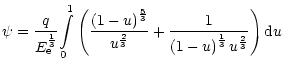
In quantum electrodynamics, the process of pair creation of photons takes
place in an external magnetic field which can absorb momentum perpendicular
to its strength B (Harding 1997). The rate of pair
creation (Toll 1952; Klepikov 1954) increases rapidly
with increasing photon
energy and transverse magnetic field strength, becoming significant for
fields approaching the critical field strength of
 G. Assuming EHE photons
emitted at very small angles to the magnetic
field (Sturrock 1971; Ruderman 1975), such photons will
convert into pairs only after traveling a distance
G. Assuming EHE photons
emitted at very small angles to the magnetic
field (Sturrock 1971; Ruderman 1975), such photons will
convert into pairs only after traveling a distance
 comparable to the field line radius of curvature
  ,
so
that
,
so
that
 where
where  is the angle between the photon momentum and magnetic
field vectors. The above results agree numerically with the analytical
expression of the one-photon pair creation rate near threshold energy
derived by Baring (1988) for a magnetic field intensity nearly equal
or exceeding the value of 0.1
is the angle between the photon momentum and magnetic
field vectors. The above results agree numerically with the analytical
expression of the one-photon pair creation rate near threshold energy
derived by Baring (1988) for a magnetic field intensity nearly equal
or exceeding the value of 0.1
 .
The rate of pair production of an EHE photon with energy
.
The rate of pair production of an EHE photon with energy
 can be expressed in terms of the attenuation
coefficient (Klepikov 1954; Tsai 1974) as:
can be expressed in terms of the attenuation
coefficient (Klepikov 1954; Tsai 1974) as:
 |
|
|
(1) |
knowing that;
 |
|
|
(2) |
where  =
=
 and
and
 (Compton wavelength
of the electron), m
(Compton wavelength
of the electron), m
 is
the electron mass.
The labels p, n of the parameter
is
the electron mass.
The labels p, n of the parameter
 refer to the state in which the photon's electric field vector
is parallel and normal to the plane (containing the magnetic field and
the photon's momentum vector) respectively.
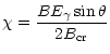
The value of that parameter
refer to the state in which the photon's electric field vector
is parallel and normal to the plane (containing the magnetic field and
the photon's momentum vector) respectively.
The value of that parameter
 for
for  1, and
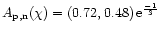 for
for
 .
.
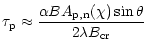
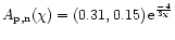
The probability of pair creation and photon
splitting for an EHE photon with energy
in
a magnetic field of strength B increases when B is at least a significant
fraction of the quantum critical field
.
The splitting rate of photon in external magnetic field is expressible
(Papanyan 1972) in terms of the splitting attenuation coefficient as:
 |
|
|
(3) |
where
 ,
,
 for
for
 and equal
 for
for
 .
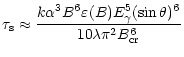
We simulated such processes using the Monte Carlo method, and Erber's rates
(Erber 1966)
were used to get the exact quantum mechanical rates for e
.
We simulated such processes using the Monte Carlo method, and Erber's rates
(Erber 1966)
were used to get the exact quantum mechanical rates for e
 pair creation by photons and photon splitting by
secondary e
pairs.
pair creation by photons and photon splitting by
secondary e
pairs.
The total probabilities per unit length (1 cm) for pair creation and photon
splitting are given by (Anguelov 1999)
 |
|
|
(4) |
where
 ,
,
 ,
,
 and
and
 are the energies of photon and electron respectively.
The above equation can be used to sample the energies of the secondary
particles such as photons in photon splitting and electrons in pair creation.
are the energies of photon and electron respectively.
The above equation can be used to sample the energies of the secondary
particles such as photons in photon splitting and electrons in pair creation.
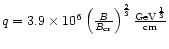
The interplanetary magnetic field of the Sun is formed as a result of the
transport of the photospheric magnetic field (Amenomori 2000) by
the solar wind flowing continuously from the Sun (Parker 1963).
Field lines
near the solar equator form closed loops (neutral sheets), while field lines
from the poles are dragged far into interplanetary space by the high-speed
solar wind.
Furthermore, the magnetic field of the Sun changes sign from south to north
across the neutral sheets. The interplanetary magnetic field can be
explained well by the Ballerina Skirt model assuming a rotating dipole in the
Sun (Schultz 1973; Saito 1975; Svalgaard 1978),
although direct evidence for the presence of such a rotating dipole has not
yet been obtained. During the solar maximum, a disturbance occurred in the solar
magnetic field due to the influence of active regions on the Sun's surface.
That field can dominate at mid to low solar latitudes (in the solar chromosphere)
by up to 2 orders of magnitude over the dipole component near the Sun, knowing
that the magnetic dipole moment of the Sun equals
 Gcm
Gcm
 .
.
We injected photons randomly with different energies in two directions (parallel
 and perpendicular
  to the
Solar Magnetic Equatorial Plane (SMEP)) within a
circle of radius
to the
Solar Magnetic Equatorial Plane (SMEP)) within a
circle of radius
 around the Sun, (where n is an integer
number ranging from 0 to 3, and
around the Sun, (where n is an integer
number ranging from 0 to 3, and
 is the Sun's radius). Magnetic
cascading initiated by primary monoenergetic photons with energies
between 10
is the Sun's radius). Magnetic
cascading initiated by primary monoenergetic photons with energies
between 10
 and 10
 eV was simulated. The primary energies of ten
simulated photons are assigned with a step of (
eV was simulated. The primary energies of ten
simulated photons are assigned with a step of (
 eV) over
the energy range, and averaged over 10 simulations.
Our simulation shows that the probability of interaction depends not only on
the primary photon energy but also on the angle of incidence. Figure 1 shows
the first interaction point (measured from
the Sun's surface) as a function of the energy of the incident primary
photons injected into the two directions mentioned before.
eV) over
the energy range, and averaged over 10 simulations.
Our simulation shows that the probability of interaction depends not only on
the primary photon energy but also on the angle of incidence. Figure 1 shows
the first interaction point (measured from
the Sun's surface) as a function of the energy of the incident primary
photons injected into the two directions mentioned before.
![\begin{figure}
\par\includegraphics[width=7.6cm,height=6.6cm,clip]{aa1723f1.eps}\end{figure}](/articles/aa/full/2002/16/aa1723/Timg56.gif) |
Figure 1:
The first interaction point for different energies of the incident primary
photons injected
(upper curve) and
(lower curve)
to the SMEP at different locations from the Sun's surface. |
| Open with DEXTER |
The figure also shows that
showers (lower curve)
start cascading at much deeper positions than
showers (upper curve) to the SMEP.
For the highest energy
showers with energy of 10
eV, cascading starts at a distance of
 from the Sun's surface; this value is reduced to
 in a case
of
showers. The difference between the two curves becomes
much wider (
in a case
of
showers. The difference between the two curves becomes
much wider (
 )
for the lowest energy showers
with primary energy 10
eV which cascade very near
to the Sun at distance
)
for the lowest energy showers
with primary energy 10
eV which cascade very near
to the Sun at distance
 from the Sun's surface. In addition,
fluctuation is much larger for the higher energy region.
from the Sun's surface. In addition,
fluctuation is much larger for the higher energy region.
![\begin{figure}
\includegraphics[width=7.5cm,height=6.7cm,clip]{aa1723f2.eps}\end{figure}](/articles/aa/full/2002/16/aa1723/Timg61.gif) |
Figure 2:
Magnetic cascading development for showers initiated by EHE photons with energies
(curves up to down) 10
,
10
,
10
 ,
10
,
10 ,
10
,
10
 ,
10 ,
10
 ,
10 ,
10
 and 10
 eV. eV. |
| Open with DEXTER |
![\begin{figure}
\par\includegraphics[width=7.5cm,height=6.7cm,clip]{aa1723f3.eps}\end{figure}](/articles/aa/full/2002/16/aa1723/Timg62.gif) |
Figure 3:
Magnetic cascading development for
showers initiated by EHE
photons with energies (curves up to down) 10
,
10
,
10
,
10
,
10
,
10
,
10
and 10
eV. |
| Open with DEXTER |
We studied the characteristics of magnetic cascading development for
showers (Fig. 2) and
showers (Fig. 3) initiated by EHE
photons.
The total number of generated photons cascading
along the path up to a given altitude from the Sun's
surface (with step of
 km) has been averaged and
plotted for the primary photons with energies
(curves from top to bottom) 10
,
10
,
10
,
10
,
10
,
10
,
10
and 10
eV.
The comparison between the two figures shows that the number of photons generated
is much higher in case of
showers than showers.
We calculated the integrated photon energy spectra of the total number
of secondary photons generated along the path up to the Sun's surface.
These results have been plotted for and
showers with step of (
km) has been averaged and
plotted for the primary photons with energies
(curves from top to bottom) 10
,
10
,
10
,
10
,
10
,
10
,
10
and 10
eV.
The comparison between the two figures shows that the number of photons generated
is much higher in case of
showers than showers.
We calculated the integrated photon energy spectra of the total number
of secondary photons generated along the path up to the Sun's surface.
These results have been plotted for and
showers with step of (
 )
and primary
energies (curves top to bottom) 10
,
10
,
10
,
10
,
10
,
10
and 10
eV
as shown in Figs. 4 and 5 respectively.
Due to computer (CPU) time limitation, the spectral analysis of the generated
secondary photons is processed for energies up to
10
)
and primary
energies (curves top to bottom) 10
,
10
,
10
,
10
,
10
,
10
and 10
eV
as shown in Figs. 4 and 5 respectively.
Due to computer (CPU) time limitation, the spectral analysis of the generated
secondary photons is processed for energies up to
10
 GeV for
showers and
10
GeV for
showers and
10
 GeV for
showers.
GeV for
showers.
![\begin{figure}
\par\includegraphics[width=6.8cm,height=6.6cm,clip]{aa1723f4.eps}\end{figure}](/articles/aa/full/2002/16/aa1723/Timg67.gif) |
Figure 4:
Integrated photon energy spectra for
showers
initiated by EHE photons with energies (curves up to down) 10
,
10
,
10
,
10
,
10
,
10
and 10
eV. |
| Open with DEXTER |
![\begin{figure}
\par\includegraphics[width=6.8cm,height=6.6cm,clip]{aa1723f5.eps}\end{figure}](/articles/aa/full/2002/16/aa1723/Timg68.gif) |
Figure 5:
Integrated photon energy spectra for
showers
initiated by EHE photons with energies (curves up to down) 10
,
10
,
10
,
10
,
10
,
10
and 10
eV. |
| Open with DEXTER |
The number of highest energy photons generated is greater in
showers than
showers, which is compatible with the
characteristics of the longitudinal development curves (see Figs. 2 and 3).
The energy weighted-spectrum for
and
showers within
the same energy levels listed before are shown in Figs. 6 and 7 respectively.
The two figures show that the energy-weighted spectrum curves for
has a maximum at a photon energy of 10
 GeV,
while this maximum appears at a photon energy of 10
GeV,
while this maximum appears at a photon energy of 10
 GeV
in the case of
showers. These can be referred to the distribution
of the highest energy particles generated through the photon energy spectra.
The electron component of the cascading is
characterized by large fluctuations and is not significant in
the cascading, therefore, the electron component is not mentioned in our results which rather
concentrate on the photon content of the cascading.
GeV
in the case of
showers. These can be referred to the distribution
of the highest energy particles generated through the photon energy spectra.
The electron component of the cascading is
characterized by large fluctuations and is not significant in
the cascading, therefore, the electron component is not mentioned in our results which rather
concentrate on the photon content of the cascading.
![\begin{figure}
\includegraphics[width=6.8cm,height=7.1cm,clip]{aa1723f6.eps}\end{figure}](/articles/aa/full/2002/16/aa1723/Timg71.gif) |
Figure 6:
The energy weighted spectrum for
showers
initiated by EHE photons with energies (curves up to down) 10
,
10
,
10
,
10
,
10
,
10
and 10
eV. |
| Open with DEXTER |
![\begin{figure}
\includegraphics[width=6.8cm,height=7.1cm,clip]{aa1723f7.eps}\end{figure}](/articles/aa/full/2002/16/aa1723/Timg72.gif) |
Figure 7:
The energy weighted spectrum for
showers
initiated by EHE photons with energies (curves up to down) 10
,
10
,
10
,
10
,
10
,
10
and 10
eV. |
| Open with DEXTER |
Our simulation shows that
showers cascade much deeper than
showers to the SMEP. This could be explained by showers having impact parameters larger than the solar radius, and
so they propagate parallel to the magnetic dipole, far away from the magnetic poles.
On the other hand, a substantial fraction of
showers
should perpendicularly cross the Sun's polar magnetic field which increases
their probability of interaction. The simulation also shows that
EHE gamma-rays with energies between 10
and
10
 eV start cascading in the Sun's
magnetic field within a circle of radius
eV start cascading in the Sun's
magnetic field within a circle of radius  times the radius of the
Sun. If we are trying to detect such cascading particles on the Earth
with air shower arrays, these showers should be detected
within a solid angle equal
times the radius of the
Sun. If we are trying to detect such cascading particles on the Earth
with air shower arrays, these showers should be detected
within a solid angle equal
 sr from the Sun's position.
The question arising now is how to distinguish such unusual showers from
ordinary showers. In the case of photons expected in the cosmic ray spectrum
above 10
eV, the answer is simply
that secondary photons of the cascades produced in the Sun's magnetosphere
arrive at the Earth's atmosphere with a significant perpendicular extent
which is the result of deflection of the paths of secondary electrons by the
Sun's magnetic field. This could be a characteristic phenomenon of such
unusual showers. In addition,
the radius of the curvature and deflection angle of such cascading showers
in the Sun's magnetic field can be simulated at the top of the Earth's
atmosphere, which will be presented in future work.
sr from the Sun's position.
The question arising now is how to distinguish such unusual showers from
ordinary showers. In the case of photons expected in the cosmic ray spectrum
above 10
eV, the answer is simply
that secondary photons of the cascades produced in the Sun's magnetosphere
arrive at the Earth's atmosphere with a significant perpendicular extent
which is the result of deflection of the paths of secondary electrons by the
Sun's magnetic field. This could be a characteristic phenomenon of such
unusual showers. In addition,
the radius of the curvature and deflection angle of such cascading showers
in the Sun's magnetic field can be simulated at the top of the Earth's
atmosphere, which will be presented in future work.
![\begin{figure}
\par\includegraphics[width=7.5cm,height=6.5cm,clip]{aa1723f8.eps}\end{figure}](/articles/aa/full/2002/16/aa1723/Timg76.gif) |
Figure 8:
The expected rate of cascading showers in the Sun's magnetic field detected
by Auger 1 and 2 experiments. |
| Open with DEXTER |
It could be helpful to estimate the expected rate of such showers
detected by the largest ground array experiments, such as the Auger experiment
in Argentina. Assuming the Auger location, the number of these showers
detected from a circle of
 around the Sun is given by:
 |
|
|
(5) |
where S is the part of the sky observed by the experiment, N is the total number
of observed showers.
Figure 8 shows the expected rate per 10 years for such showers to be detected by
the planned experiments Auger 1 and 2 with total areas of 3000 km and
7000 km
respectively. Although the predicted rate of such showers
is very small (about 1.2 and 3 showers per 10 years for Auger1 and 2), it is
possible to enlarge the detecting area by extending the detector spacing up
to 3 km to observe this kind of EHE shower in the future.
and
7000 km
respectively. Although the predicted rate of such showers
is very small (about 1.2 and 3 showers per 10 years for Auger1 and 2), it is
possible to enlarge the detecting area by extending the detector spacing up
to 3 km to observe this kind of EHE shower in the future.
Acknowledgements
The authors would like to thank Prof. H. Vankov for his useful comments and
discussions.
- Amenomori, M., et al. 2000, Phys. Rep. [astro-ph/0008159]
In the text
- Anguelov, V., & Vankov, H. 1999, J. Phys. G: Nucl. Part. Physics, 251, 10
In the text
- Baring, M. G. 1988, MNRAS, 235, 79
In the text
NASA ADS
- Bednarek, W. 1999, Astro Phys. [astro-ph/9911266]
In the text
- Bhattacharjee, P., & Sigl 1999, Phys. Rep. [astro-ph/9811011]
In the text
- Bird, D. J., Corbató, S. C., Dai, H. Y., et al. 1993, Phys. Rev. Lett., 71, 3401
In the text
NASA ADS
- Erber, T. 1966, Rev. Mod. Phys., 38, 626
In the text
- Halzen, F., Protheroe, R. J., Stanev, T., Vankov, H. P., et al. 1990, Phys. Rev. D, 41, 342
In the text
NASA ADS
- Hillas, A. M. 1984, ARA, 22, 425
In the text
- Harding, A. K., & Baring, M. G. 1997, ApJ, 476, 246
In the text
NASA ADS
- Klepikov, N. V. 1954, Zh. Eksp. Theor. Fiz., 26, 19, first citation in article
In the text
- Papanyan, V. O., & Ritus, V. I. 1972, Sov. Phys., 34, 1195
In the text
- Parker, E. J. 1963, Interplanetary Dynamical Process (New York: Interscience)
In the text
- Ruderman, M. A., & Sutherland, P. G. 1975, ApJ, 196, 51
In the text
NASA ADS
- Saito, T. 1975, Sci. Rep. Tohoku Univ., Ser., 5, 23, 37
In the text
- Schultz, M. 1973, Astrophys. Space Sci., 24, 371
In the text
- Sturrock, P. A. 1971, ApJ, 164, 529
In the text
NASA ADS
- Svalgaard, L., & Wilcox, J. M. 1978, ARA&A, 16, 429
In the text
NASA ADS
- Toll, J. S. 1952, Ph.D. Thesis, Princeton Univ., first citation in article
In the text
- Tsai, W. Y., & Erber, T. 1974, Phys. Rev. D, 10, 492
In the text
NASA ADS
- Wdowczyk, J., & Wolfendale, A. W. 1990, ApJ, 349, 35
In the text
NASA ADS
Copyright ESO 2002
![\begin{figure}
\par\includegraphics[width=7.6cm,height=6.6cm,clip]{aa1723f1.eps}\end{figure}](/articles/aa/full/2002/16/aa1723/img56.gif)
![\begin{figure}
\includegraphics[width=7.5cm,height=6.7cm,clip]{aa1723f2.eps}\end{figure}](/articles/aa/full/2002/16/aa1723/img61.gif)
![\begin{figure}
\par\includegraphics[width=7.5cm,height=6.7cm,clip]{aa1723f3.eps}\end{figure}](/articles/aa/full/2002/16/aa1723/img62.gif)
![\begin{figure}
\par\includegraphics[width=6.8cm,height=6.6cm,clip]{aa1723f4.eps}\end{figure}](/articles/aa/full/2002/16/aa1723/img67.gif)
![\begin{figure}
\par\includegraphics[width=6.8cm,height=6.6cm,clip]{aa1723f5.eps}\end{figure}](/articles/aa/full/2002/16/aa1723/img68.gif)
![\begin{figure}
\includegraphics[width=6.8cm,height=7.1cm,clip]{aa1723f6.eps}\end{figure}](/articles/aa/full/2002/16/aa1723/img71.gif)
![\begin{figure}
\includegraphics[width=6.8cm,height=7.1cm,clip]{aa1723f7.eps}\end{figure}](/articles/aa/full/2002/16/aa1723/img72.gif)
![\begin{figure}
\par\includegraphics[width=7.5cm,height=6.5cm,clip]{aa1723f8.eps}\end{figure}](/articles/aa/full/2002/16/aa1723/img76.gif)