A&A 385, 572-584 (2002)
DOI: 10.1051/0004-6361:20020137
J. De Ridder 1 - M.-A. Dupret 2 - C. Neuforge 2 - C. Aerts 1
1 -
Instituut voor Sterrenkunde, Katholieke Universiteit
Leuven, Celestijnenlaan 200 B, 3001 Heverlee, Belgium
2 -
Institut d'Astrophysique et de Géophysique de
l'Université de Liège, avenue de Cointe 5, 4000 Liège, Belgium
Received 2 August 2001 / Accepted 23 January 2002
Abstract
We investigate to what extent non-adiabatic temperature variations
at the
surface of slowly rotating non-radially pulsating ![]() Cephei stars and
slowly pulsating B stars affect silicon line profile variations. We use the
non-adiabatic amplitudes of the effective temperature and gravity
variation presented in Dupret et al. (2002), together with a Kurucz
intensity grid, to compute time series of line profile variations.
Our simulations point out that the line shapes do not change significantly
due to temperature variations. We find equivalent width variations of at
most two percent of the mean equivalent width.
We confront our results with observational equivalent width
variations and with photometrically obtained effective temperature variations.
Cephei stars and
slowly pulsating B stars affect silicon line profile variations. We use the
non-adiabatic amplitudes of the effective temperature and gravity
variation presented in Dupret et al. (2002), together with a Kurucz
intensity grid, to compute time series of line profile variations.
Our simulations point out that the line shapes do not change significantly
due to temperature variations. We find equivalent width variations of at
most two percent of the mean equivalent width.
We confront our results with observational equivalent width
variations and with photometrically obtained effective temperature variations.
Key words: stars: early-type - stars: variables: ![]() Cep -
stars: variables: slowly pulsating B stars - line: profiles
Cep -
stars: variables: slowly pulsating B stars - line: profiles
Since the pioneering work of Osaki, there has always been a keen interest in line profile modelling. After all, one can expect that time series of stellar spectra contain more pulsational information than any other observable. Moreover, since the beginning of the 1980s the spectroscopic resolution greatly improved so that LPVs can be studied in much detail. LPVs have been used, for example, to study the influence of rotation on pulsation (e.g. Lee & Saio 1990), to distinguish between non-radial pulsation and spots (e.g. Briquet et al. 2001) or to perform a mode identification via line profile fitting (e.g. Smith & Buta 1979), via the moments of the line profile (e.g. Aerts et al. 1994) or via the Doppler imaging technique (e.g. Telting & Schrijvers 1997). For each of these applications of line profile modelling, it is vital to have a profound understanding of the physics behind the line profile variations. Failing to recognize some of the relevant aspects of LPVs can lead to invalid conclusions.
A problem that is still not satisfactorily settled, is whether temperature
variations at the surface of a non-radially pulsating star play an important
role in shaping the line profiles.
It is well known that, during the pulsation cycle, the temperature and the
other thermodynamical quantities like P and ![]() ,
are varying with time.
This leads to intensity variations both in the continuum and the local line
profile.
The question is how much this affects the normalized disk integrated flux
line profiles. Could, for example, neglecting the temperature variations
in the case of line profile fitting, jeopardize a mode identification?
,
are varying with time.
This leads to intensity variations both in the continuum and the local line
profile.
The question is how much this affects the normalized disk integrated flux
line profiles. Could, for example, neglecting the temperature variations
in the case of line profile fitting, jeopardize a mode identification?
The fact that the effects of temperature variations cannot just be ignored without further investigation, was realized by several authors, be it mainly for rapidly rotating pulsators because the effects are expected to be most pronounced for these stars. Balona (1987) tried to mimick the effects of temperature variations on the moments of a line profile by introducing an artificial extra velocity field. Lee & Saio (1990), using a constant gaussian as local line profile, included a temperature dependent continuum intensity. Lee et al. (1992) extended this work by including equivalent width variations in their model. Schrijvers & Telting (1999) also used in their model a gaussian local line profile with a temperature dependent continuum and equivalent width to see the impact on the performance of the Doppler imaging mode identification technique. Cugier (1993) and Townsend (1997) used a somewhat more advanced temperature dependent local line profile. The essential conclusion of all these authors is basically the same: temperature variations may have a large influence on LPVs. However, the weak point in their investigations is the unknown amplitude of the temperature variation. Often the temperature variations are computed in the adiabatic approach, with an arbitrary free parameter to correct for non-adiabaticity in the photosphere.
In our investigations, we concentrated on ![]() Cephei stars
and SPBs. Some of them are slow rotators, and are therefore currently
the more simple (though still difficult!) cases for mode identification,
because the velocity field can be well described by one spherical harmonic
Cephei stars
and SPBs. Some of them are slow rotators, and are therefore currently
the more simple (though still difficult!) cases for mode identification,
because the velocity field can be well described by one spherical harmonic
![]() .
In Dupret et al. (2002, Paper I), non-adiabatic eigenfunctions
in the atmospheres
of non-rotating non-radially pulsating B stars have been presented.
We here present line-profile simulations based on these eigenfunctions.
Our main concern was to investigate how local effective temperature
variations affect the LPVs of these kinds of stars.
.
In Dupret et al. (2002, Paper I), non-adiabatic eigenfunctions
in the atmospheres
of non-rotating non-radially pulsating B stars have been presented.
We here present line-profile simulations based on these eigenfunctions.
Our main concern was to investigate how local effective temperature
variations affect the LPVs of these kinds of stars.
![\begin{figure}
\par\includegraphics[angle=270,width=8.5cm,clip]{3069f1.eps}
\end{figure}](/articles/aa/full/2002/14/aah3069/img37.gif) |
Figure 1:
Relative effective temperature variation as a function of the average
effective temperature for SPBs (open circles) and |
| Open with DEXTER | |
We should be careful with the interpretation of the results presented in
Fig. 1: what does an effective temperature mean in the case of a
non-radial (and therefore non-spherically symmetric) pulsator?
The radiation intensity at the surface of a non-radially
pulsating star has an angular dependence due to the pulsation. The
disk-integrated flux we observe, is therefore a weighted average,
and the derived
![]() should also be considered as a weighted average. The amplitudes
of the
should also be considered as a weighted average. The amplitudes
of the
![]() variations of the local atmospheres (see Paper I) are
therefore higher. We also recall that the
variations of the local atmospheres (see Paper I) are
therefore higher. We also recall that the
![]() calibration of Künzli et al. (1997) involved computing synthetic photometric
colours with static LTE Kurucz models which are subsequently corrected with
standard stars to match better the observations. The B stars among these
standard stars contained (inevitably) non-radial pulsators.
calibration of Künzli et al. (1997) involved computing synthetic photometric
colours with static LTE Kurucz models which are subsequently corrected with
standard stars to match better the observations. The B stars among these
standard stars contained (inevitably) non-radial pulsators.
From Fig. 1 it follows that SPBs appear to have a somewhat
lower
![]() variability
than
variability
than ![]() Cephei stars, but the sample sizes are too small to make this
conclusion firm. Figure 2 shows examples of targets for
which a clear sinusoidal
Cephei stars, but the sample sizes are too small to make this
conclusion firm. Figure 2 shows examples of targets for
which a clear sinusoidal
![]() variation could be found. We include
these phase diagrams to show what kind of amplitudes of
variation could be found. We include
these phase diagrams to show what kind of amplitudes of
![]() can be detected if the quality of the data is sufficiently high
and if the star has a dominant pulsation mode.
We conclude that the
can be detected if the quality of the data is sufficiently high
and if the star has a dominant pulsation mode.
We conclude that the
![]() can vary by several hundred Kelvin and
that this should be considered as a lower limit for the
can vary by several hundred Kelvin and
that this should be considered as a lower limit for the
![]() variation of the local atmosphere.
variation of the local atmosphere.
![\begin{figure}
\par\includegraphics[angle=270,width=13.5cm,clip]{3069f2.eps}
\end{figure}](/articles/aa/full/2002/14/aah3069/img38.gif) |
Figure 2:
The upper panel shows the real-time variation of the effective
temperature
|
| Open with DEXTER | |
In this section, as well as in the remainder of the paper, we will
concentrate on silicon lines: the SiII doublet around 413 nm and the
SiIII triplet around 456 nm. The former are pronouncedly present in SPBs, the
latter in ![]() Cephei stars. Being neither too weak nor too strong in
almost
the entire instability strip where they are used, these Si-lines are often
used to study LPVs and identify the modes in pulsating B stars (see
e.g. Aerts et al. 1994; Aerts et al. 1999). This
spectral line selection criterion implies that their
Cephei stars. Being neither too weak nor too strong in
almost
the entire instability strip where they are used, these Si-lines are often
used to study LPVs and identify the modes in pulsating B stars (see
e.g. Aerts et al. 1994; Aerts et al. 1999). This
spectral line selection criterion implies that their
![]() dependence is not extremely strong. We will check in this paper whether these
lines are sufficiently insensitive to
dependence is not extremely strong. We will check in this paper whether these
lines are sufficiently insensitive to
![]() variations to be modeled
in slowly rotating pulsators without any incorporation of temperature
variations as is done in e.g. the moment method (Aerts et al. 1992)
variations to be modeled
in slowly rotating pulsators without any incorporation of temperature
variations as is done in e.g. the moment method (Aerts et al. 1992)
![\begin{figure}
\par\includegraphics[angle=270,width=7.8cm,clip]{3069f3.eps}
\end{figure}](/articles/aa/full/2002/14/aah3069/img39.gif) |
Figure 3:
Relative EW variation as a function of the average
effective temperature for SPBs (open circles) and |
| Open with DEXTER | |
![\begin{figure}
\par\includegraphics[angle=270,width=12.3cm,clip]{3069f4a.eps}\pa...
...*{3.5mm}
\includegraphics[angle=270,width=12.3cm,clip]{3069f4b.eps}
\end{figure}](/articles/aa/full/2002/14/aah3069/img42.gif) |
Figure 4:
EW and radial velocity phase diagrams of the
two |
| Open with DEXTER | |
We remark that the equivalent width variations of different lines
need not be in phase.
For example, the EW variation of He lines in an SPB are in antiphase with
the EW variations of the SiII doublet (De Cat, private communication).
The reason is that, as is well known, the
![]() )
curve has an
ascending branch, a top, and a descending branch. For SPBs the SiII doublet
is situated in the descending branch of the
)
curve has an
ascending branch, a top, and a descending branch. For SPBs the SiII doublet
is situated in the descending branch of the
![]() )
curve while the
He lines are situated in the ascending branch.
)
curve while the
He lines are situated in the ascending branch.
Non-adiabatic computations predict a small extra phase shift between
the EW and the observed radial velocity
![]() .
Observationally however, it is difficult to measure this phase
lag because of noise and multiperiodicity.
.
Observationally however, it is difficult to measure this phase
lag because of noise and multiperiodicity.
The length of the vector
![]() measures the area of the
surface element, so that the projected area
measures the area of the
surface element, so that the projected area ![]() can be computed from
can be computed from
![]() .
With
.
With
![]() ,
we denote the cosine of the angle between the local surface normal and the
observer's vector:
,
we denote the cosine of the angle between the local surface normal and the
observer's vector:
![]() .
The quantity
.
The quantity ![]() is needed to compute the radiation intensity in the
direction of the observer as well as to determine whether a surface element is
visible or not. The latter is done by checking the sign of
is needed to compute the radiation intensity in the
direction of the observer as well as to determine whether a surface element is
visible or not. The latter is done by checking the sign of ![]() :
an element is
visible when
:
an element is
visible when ![]() is positive and invisible when
is positive and invisible when ![]() is negative.
is negative.
The temperature effects on the line-profile variations
are taken into account through the variation of the local
![]() ,
and not through the Lagrangian variation
of the temperature at the line forming optical depth.
As shown in Paper I, it can be argued that at time t the temperature
distribution of the perturbed local atmosphere is well approximated by the
temperature distribution of an equilibrium model.
For the same physical reasons, we assume that the intensity
field of the perturbed local atmosphere
is also well approximated by the intensity field of an
equilibrium atmosphere model. And since for a given metallicity,
the latter only depends on the quantities
,
and not through the Lagrangian variation
of the temperature at the line forming optical depth.
As shown in Paper I, it can be argued that at time t the temperature
distribution of the perturbed local atmosphere is well approximated by the
temperature distribution of an equilibrium model.
For the same physical reasons, we assume that the intensity
field of the perturbed local atmosphere
is also well approximated by the intensity field of an
equilibrium atmosphere model. And since for a given metallicity,
the latter only depends on the quantities
![]() and
and ![]() ,
it is appropriate to use
,
it is appropriate to use
![]() and
and
![]() as variables in our simulations.
as variables in our simulations.
Although, as mentioned earlier, PULSTAR allows to include rotational broadening, the latter was always taken zero in the following sections.
To have an idea about the range of line forming layers, we adopt a new
approach. Consider, as an example, the line contribution function
![]() for the SiIII (456.784 nm) line, as
shown in Fig. 5.
for the SiIII (456.784 nm) line, as
shown in Fig. 5.
![\begin{figure}
\par\includegraphics[width=8.5cm,clip]{3069f5.eps}
\end{figure}](/articles/aa/full/2002/14/aah3069/img101.gif) |
Figure 5:
The line contribution function CU as a function
of the wavelength |
| Open with DEXTER | |
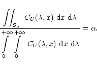 |
(5) |
| (6) | |||
| (7) |
Our results for the SiIII (456.784 nm) line in the case of the ![]() Cephei
model and the SiII (412.805 nm) line in the case of the SPB model can be found
in Figs. 6 and 7.
These figures show that the most contributing layer
is
Cephei
model and the SiII (412.805 nm) line in the case of the SPB model can be found
in Figs. 6 and 7.
These figures show that the most contributing layer
is
![]() for the SiIII line and
for the SiIII line and
![]() for the
SiII line. We used these layers to evaluate the quantities (2), (3) and (4).
for the
SiII line. We used these layers to evaluate the quantities (2), (3) and (4).
![\begin{figure}
\par\includegraphics[angle=270,width=8.4cm,clip]{3069f6.eps}
\end{figure}](/articles/aa/full/2002/14/aah3069/img118.gif) |
Figure 6:
Upper and lower end of the line forming range of the SiIII
(456.784 nm) line for the |
| Open with DEXTER | |
![\begin{figure}
\par\includegraphics[angle=270,width=8.4cm,clip]{3069f7.eps}
\end{figure}](/articles/aa/full/2002/14/aah3069/img119.gif) |
Figure 7: Same as in Fig. 6 but for the SiII (412.805 nm) line for the SPB atmosphere model mentioned in Paper I. |
| Open with DEXTER | |
One should be aware that we are using the range of line formation computed
with CU, as the range of line formation for the relative
flux depression. It is unclear how accurate this approximation is.
For the Si lines under consideration (in MS B star spectra),
we verified whether
![\begin{figure}
\par\includegraphics[angle=270,width=8.3cm,clip]{3069f8.eps}
\end{figure}](/articles/aa/full/2002/14/aah3069/img120.gif) |
Figure 8:
The variation of |
| Open with DEXTER | |
![\begin{figure}
\includegraphics[angle=270,width=8.3cm,clip]{3069f9.eps}
\end{figure}](/articles/aa/full/2002/14/aah3069/img121.gif) |
Figure 9:
Same as in Fig. 8 but for the SiII (412.805 nm)
line and for the SPB modes listed in Table 2.
The triangles denote |
| Open with DEXTER | |
Although the line forming ranges, given an ![]() ,
are ranges for a static
atmosphere, we have a priori no reason to believe that these ranges will
be smaller for a dynamic atmosphere.
It is therefore interesting to check how much
,
are ranges for a static
atmosphere, we have a priori no reason to believe that these ranges will
be smaller for a dynamic atmosphere.
It is therefore interesting to check how much ![]() and
and ![]() change over the line forming range, in order to see how good
the commonly used one-layer model is. From Figs. 6 and
7 one can see that the 90% contribution range in
change over the line forming range, in order to see how good
the commonly used one-layer model is. From Figs. 6 and
7 one can see that the 90% contribution range in ![]() is
[-2.875, -0.125] for the SiIII line and
[-3.625, 0.250] for the SiII line.
The variations of
is
[-2.875, -0.125] for the SiIII line and
[-3.625, 0.250] for the SiII line.
The variations of ![]() and
and ![]() over the line forming range were
estimated by computing (s - d)/d where s stands for the value in the
shallower end of the range and d for the deeper end of the range. The
results for the different pulsation modes listed in Tables 1 and
2 are shown in Figs. 8 and 9.
From these figures it can be immediately seen that for some modes, the
one-layer approximation is a rather crude one, in the sense that the
eigenfunctions
over the line forming range were
estimated by computing (s - d)/d where s stands for the value in the
shallower end of the range and d for the deeper end of the range. The
results for the different pulsation modes listed in Tables 1 and
2 are shown in Figs. 8 and 9.
From these figures it can be immediately seen that for some modes, the
one-layer approximation is a rather crude one, in the sense that the
eigenfunctions ![]() and
and ![]() vary quite a lot in the line forming
region so that assigning a single value to these quantities may be
inappropriate. Remarkable is also that the one-layer approximation is often
better for the high-order g-modes of the SPB model than for the low-order
p-modes of the
vary quite a lot in the line forming
region so that assigning a single value to these quantities may be
inappropriate. Remarkable is also that the one-layer approximation is often
better for the high-order g-modes of the SPB model than for the low-order
p-modes of the ![]() Cephei model. It is still unclear, however, how good
the one-layer
approximation is to compute LPVs. Probably the only way to find out is
to compute time series of line profiles with a spectral line synthesis
code suitable for the dynamic atmospheres of non-radially pulsating stars.
Such an approach, however, is currently beyond our scope.
Evaluating the eigenfunctions in a "mean layer'' somehow
defined as a weighted average of the line forming layers, would not
yield much additional insight since the essential physics (e.g. a different
velocity field for the line core than for the line wings) would still not be
present. Since the wings are formed deeper in the atmosphere than the core,
and because the amplitude of the displacement (and thus the velocity)
increases towards the surface, and because the "one'' layer we use is the
core-forming layer, we can expect that the Doppler shift of the line wings
is overestimated.
Cephei model. It is still unclear, however, how good
the one-layer
approximation is to compute LPVs. Probably the only way to find out is
to compute time series of line profiles with a spectral line synthesis
code suitable for the dynamic atmospheres of non-radially pulsating stars.
Such an approach, however, is currently beyond our scope.
Evaluating the eigenfunctions in a "mean layer'' somehow
defined as a weighted average of the line forming layers, would not
yield much additional insight since the essential physics (e.g. a different
velocity field for the line core than for the line wings) would still not be
present. Since the wings are formed deeper in the atmosphere than the core,
and because the amplitude of the displacement (and thus the velocity)
increases towards the surface, and because the "one'' layer we use is the
core-forming layer, we can expect that the Doppler shift of the line wings
is overestimated.
It is also interesting to understand the qualitative nature of
Figs. 8 and 9. It can be seen that the
variation of ![]() and
and ![]() increases with increasing frequency
for the
increases with increasing frequency
for the ![]() Cephei star modes, but decreases with increasing
frequency for the SPB modes. This is because for p-modes the number of
radial nodes of the displacement eigenfunction increases with increasing
frequency. As a consequence, for increasing frequency, the "last'' node
gets closer to the surface, so that the derivative of
Cephei star modes, but decreases with increasing
frequency for the SPB modes. This is because for p-modes the number of
radial nodes of the displacement eigenfunction increases with increasing
frequency. As a consequence, for increasing frequency, the "last'' node
gets closer to the surface, so that the derivative of ![]() and
and
![]() is larger in the atmosphere. For g-modes, as is well known,
the number of radial nodes decreases with increasing frequency so that the
opposite effect happens. For p-modes, the variation of
is larger in the atmosphere. For g-modes, as is well known,
the number of radial nodes decreases with increasing frequency so that the
opposite effect happens. For p-modes, the variation of
![]() and
and ![]() for different degrees
for different degrees ![]() form one curve,
while for g-modes there are clearly three different curves. This can be
understood as follows. Close to the surface of the star, the system of
equations describing non-adiabatic non-radial oscillations, mainly depend on
the degree
form one curve,
while for g-modes there are clearly three different curves. This can be
understood as follows. Close to the surface of the star, the system of
equations describing non-adiabatic non-radial oscillations, mainly depend on
the degree ![]() through the conservation of mass equation (Eq. (21)
of Paper I) which contains a term with the factor
through the conservation of mass equation (Eq. (21)
of Paper I) which contains a term with the factor
![]() associated
to the transversal compression. For low-degree p-modes with a relative
high frequency, this term is very small. Therefore, for a given frequency, the
r-dependent part of the pulsation eigenfunctions does
not depend on the degree
associated
to the transversal compression. For low-degree p-modes with a relative
high frequency, this term is very small. Therefore, for a given frequency, the
r-dependent part of the pulsation eigenfunctions does
not depend on the degree ![]() in the atmosphere in a good approximation.
On the other hand, for low-frequency g-modes this term is very significant,
so that in the atmosphere the pulsation eigenfunctions of g-modes do
depend on the degree
in the atmosphere in a good approximation.
On the other hand, for low-frequency g-modes this term is very significant,
so that in the atmosphere the pulsation eigenfunctions of g-modes do
depend on the degree ![]() .
.
The parameters K, fT, ![]() ,
fg and
,
fg and ![]() are listed in Tables 1 and 2 and were computed, as explained
in Paper I, with a non-adiabatic pulsation code with special care for the
stellar atmosphere. Since this code was written for non-rotating stars,
these parameters are independent of m.
The periods of the modes can also be found in Paper I.
The azimuthal number m was varied each time from 0 to
are listed in Tables 1 and 2 and were computed, as explained
in Paper I, with a non-adiabatic pulsation code with special care for the
stellar atmosphere. Since this code was written for non-rotating stars,
these parameters are independent of m.
The periods of the modes can also be found in Paper I.
The azimuthal number m was varied each time from 0 to ![]() .
This resulted
in 49 different modes for the
.
This resulted
in 49 different modes for the ![]() Cephei model and 59 different modes for
the SPB model.
Cephei model and 59 different modes for
the SPB model.
Next, we turn to the choice of the pulsation amplitude afor each mode. Given a value for fT, the amplitude
of
![]() is scaled to the amplitude a of the
radial displacement. An unrealistically high value of the latter therefore
implies extreme temperature variations,
which will undoubtfully show a large but
meaningless effect on the LPVs. On the other hand, we
should not choose a too small because we wish to know the effect on line
profiles in the worst (but still realistic) case.
We considered two ways to set the amplitude. One way is to take for each
mode a different amplitude a in such a way that the maximum length of the
pulsational velocity vector
is scaled to the amplitude a of the
radial displacement. An unrealistically high value of the latter therefore
implies extreme temperature variations,
which will undoubtfully show a large but
meaningless effect on the LPVs. On the other hand, we
should not choose a too small because we wish to know the effect on line
profiles in the worst (but still realistic) case.
We considered two ways to set the amplitude. One way is to take for each
mode a different amplitude a in such a way that the maximum length of the
pulsational velocity vector
![]() is the same
for each mode, which is also done by e.g. Townsend (1997). Another way is to
take for each mode a different amplitude a in such a way that the maximum
length of the relative displacement vector
is the same
for each mode, which is also done by e.g. Townsend (1997). Another way is to
take for each mode a different amplitude a in such a way that the maximum
length of the relative displacement vector
![]() is the
same for each mode. Since the maximum value of
is the
same for each mode. Since the maximum value of
![]() depends on the
quantum numbers
depends on the
quantum numbers ![]() ,
both ways also allow for a better comparison
between LPVs coming from different sets of
,
both ways also allow for a better comparison
between LPVs coming from different sets of ![]() .
Of course, one should avoid amplitudes that would cause shock waves or an
unreasonably distorted surface. For this purpose, it seems more natural to fix
.
Of course, one should avoid amplitudes that would cause shock waves or an
unreasonably distorted surface. For this purpose, it seems more natural to fix
![]() for SPBs and to fix
for SPBs and to fix
![]() for
for ![]() Cephei stars, because of
the difference in magnitude of their pulsation frequencies. Indeed, for
SPBs "reasonable'' velocities can still lead to displacements out
of the linear regime while the opposite is true for the
Cephei stars, because of
the difference in magnitude of their pulsation frequencies. Indeed, for
SPBs "reasonable'' velocities can still lead to displacements out
of the linear regime while the opposite is true for the ![]() Cephei stars.
The chosen values of
Cephei stars.
The chosen values of
![]() or
or
![]() will be given in the following sections.
will be given in the following sections.
A final input parameter that needs discussion is the inclination angle iwhich affects both the line profile variability and the influence of
temperature variations on the line profile, because of cancellation effects.
For example, the amplitude of the observed radial velocity
![]() strongly depends on the inclination angle. In fact, as
explained in Chadid et al. (2001), for each non-radial mode there exists at
least one so-called inclination angle of complete cancellation ( IACC)
for which the amplitude of
strongly depends on the inclination angle. In fact, as
explained in Chadid et al. (2001), for each non-radial mode there exists at
least one so-called inclination angle of complete cancellation ( IACC)
for which the amplitude of
![]() is exactly zero.
In an analoguous way as in Chadid et al. (2001), one can also compute the
inclination angle for which the amplitude of
is exactly zero.
In an analoguous way as in Chadid et al. (2001), one can also compute the
inclination angle for which the amplitude of
![]() reaches its
maximum. We call such an angle "inclination angle of least
cancellation''
( IALC). We restrict ourselves in the simulation to inclination angles
which are IALCs as the temperature effects are largest for them, and we
list them in Table 3. A mode
reaches its
maximum. We call such an angle "inclination angle of least
cancellation''
( IALC). We restrict ourselves in the simulation to inclination angles
which are IALCs as the temperature effects are largest for them, and we
list them in Table 3. A mode ![]() can have several IALCs (i.e. several global maxima),
but we systematically used the lowest one.
can have several IALCs (i.e. several global maxima),
but we systematically used the lowest one.
For the ![]() Cephei model we set the amplitude a by fixing
Cephei model we set the amplitude a by fixing
![]() to 20 km s-1 for every mode.
The amplitudes of the radial velocities
to 20 km s-1 for every mode.
The amplitudes of the radial velocities
![]() of the modes with degree
of the modes with degree ![]() 1, 2, 3, and 4 are then respectively about
11 km s-1, 7 kms-1, 3 km s-1 and 0.5 km s-1.
The maximum length of the relative displacement vector,
1, 2, 3, and 4 are then respectively about
11 km s-1, 7 kms-1, 3 km s-1 and 0.5 km s-1.
The maximum length of the relative displacement vector,
![]() ,
was always smaller than 1%.
Most of the spectroscopically observed non-radially pulsating
,
was always smaller than 1%.
Most of the spectroscopically observed non-radially pulsating
![]() Cephei stars have an amplitude of
Cephei stars have an amplitude of
![]() smaller than
11 km s-1. Some
smaller than
11 km s-1. Some ![]() Cephei stars with a radial first mode are
known to have a larger
Cephei stars with a radial first mode are
known to have a larger
![]() amplitude, e.g.
amplitude, e.g. ![]() Cephei, the
prototype star itself, shows a radial velocity variation with an amplitude of
about 14 kms-1 (Aerts et al. 1994).
Cephei, the
prototype star itself, shows a radial velocity variation with an amplitude of
about 14 kms-1 (Aerts et al. 1994).
| mode | K | fT | fg | |||
|
|
0.05 | 2.93 | 179 |
21.0 | 180 |
|
| 0.04 | 3.26 | 187 |
26.7 | 180 |
||
| 0.03 | 3.54 | 195 |
33.3 | 180 |
||
|
|
0.04 | 3.27 | 186 |
26.4 | 180 |
|
| 0.03 | 3.43 | 191 |
30.2 | 180 |
||
| 0.02 | 3.62 | 199 |
36.7 | 180 |
||
| 0.02 | 3.66 | 212 |
47.5 | 180 |
||
|
|
0.03 | 3.43 | 190 |
29.4 | 180 |
|
| 0.02 | 3.69 | 203 |
39.8 | 180 |
||
| 0.02 | 3.71 | 209 |
45.0 | 180 |
||
| 0.02 | 3.59 | 216 |
51.1 | 180 |
||
|
|
0.03 | 3.59 | 195 |
33.3 | 180 |
|
| 0.02 | 3.72 | 205 |
42.4 | 180 |
||
| 0.01 | 3.50 | 219 |
53.8 | 180 |
| mode | K | fT | fg | |||
|
|
17.5 | 3.62 | 319 |
2.00 | 180 |
|
| 24.6 | 5.68 | 327 |
1.95 | 180 |
||
| 36.1 | 8.54 | 336 |
1.89 | 180 |
||
| 50.0 | 11.2 | 343 |
1.86 | 180 |
||
| 66.7 | 13.6 | 349 |
1.79 | 180 |
||
| 86.1 | 15.4 | 354 |
1.73 | 180 |
||
| 108 | 16.9 | 357 |
1.66 | 180 |
||
|
|
12.9 | 6.94 | 329 |
1.95 | 180 |
|
| 17.9 | 9.89 | 337 |
1.88 | 180 |
||
| 23.2 | 12.4 | 343 |
1.81 | 180 |
||
| 30.3 | 14.8 | 349 |
1.74 | 180 |
||
| 38.3 | 16.8 | 353 |
1.68 | 180 |
||
| 47.0 | 18.4 | 357 |
1.61 | 180 |
||
| 58.3 | 19.9 | 0 |
1.53 | 180 |
||
|
|
11.6 | 10.7 | 339 |
1.87 | 180 |
|
| 15.2 | 13.5 | 345 |
1.79 | 180 |
||
| 19.2 | 15.8 | 350 |
1.71 | 180 |
||
| 23.6 | 17.8 | 354 |
1.63 | 180 |
||
| 29.2 | 19.6 | 358 |
1.55 | 180 |
||
| 35.7 | 21.2 | 0 |
1.45 | 180 |
| IALC | m = 0 | m = 1 | m = 2 | m = 3 | m = 4 |
| 0 |
90 |
||||
| 0 |
45 |
90 |
|||
| 0 |
31.1 |
54.7 |
90 |
||
| 0 |
23.9 |
40.9 |
60 |
90 |
A first result of the simulations is that - with the realistic amplitudes
given above - the non-adiabatic relative temperature variation
and the relative gravity variation seem to have very little effect on
the line profiles.
The relative difference in residual intensity between a line profile computed
with and without
![]() and
and ![]() variations is always about 1% or
less. To visualize for the SiIII (456.784 nm) line this difference in
residual intensity for each wavelength in the line and at each phase during
the pulsation cycle, we computed for the p1 modes
variations is always about 1% or
less. To visualize for the SiIII (456.784 nm) line this difference in
residual intensity for each wavelength in the line and at each phase during
the pulsation cycle, we computed for the p1 modes
![]() and
and
![]() greyscale plots which are shown in the upper panels of
Fig. 10. The abscissa shows the wavelength in nanometer,
and the ordinate shows the pulsation phase between 0 and 1.
The input parameters are the same as mentioned above, in particular the
inclination angle is an IALC. White indicates a positive difference in
residual intensity, black a negative difference. The
plots can be understood as follows. For the
greyscale plots which are shown in the upper panels of
Fig. 10. The abscissa shows the wavelength in nanometer,
and the ordinate shows the pulsation phase between 0 and 1.
The input parameters are the same as mentioned above, in particular the
inclination angle is an IALC. White indicates a positive difference in
residual intensity, black a negative difference. The
plots can be understood as follows. For the
![]() mode, we look
pole-on so that we only see the northern hemisphere. The nodal line of the
radial displacement coincides with the equator which is the edge of the visible
disk. At phase zero, the northern
hemisphere is maximally expanded so that the velocity is everywhere zero which
is why the spectral line is centered around its laboratory wavelength. At the
same time the local
mode, we look
pole-on so that we only see the northern hemisphere. The nodal line of the
radial displacement coincides with the equator which is the edge of the visible
disk. At phase zero, the northern
hemisphere is maximally expanded so that the velocity is everywhere zero which
is why the spectral line is centered around its laboratory wavelength. At the
same time the local
![]() ,
and therefore also the local EW,
is everywhere
lower than the equilibrium value. This results in a spectral line with
at each wavelength a higher
residual intensity than its counterpart computed without temperature effects.
At phase 0.5, the situation is reversed. The northern
hemisphere is now maximally compressed so that the local EW is everywhere higher
than the equilibrium value which results in a spectral line with a lower
residual intensity. For the
,
and therefore also the local EW,
is everywhere
lower than the equilibrium value. This results in a spectral line with
at each wavelength a higher
residual intensity than its counterpart computed without temperature effects.
At phase 0.5, the situation is reversed. The northern
hemisphere is now maximally compressed so that the local EW is everywhere higher
than the equilibrium value which results in a spectral line with a lower
residual intensity. For the
![]() = (1,1) mode, we look equator-on. At
phase zero the nodal line of the radial displacement, and therefore also of
= (1,1) mode, we look equator-on. At
phase zero the nodal line of the radial displacement, and therefore also of
![]() ,
coincides with the edge of the disk. The nodal line of
the radial component of the pulsational velocity, however, coincides then
with the meridian through the center of the disk. Half of the disk is receding
from us, half of the disk is approaching towards us. This averages out so that
the observed spectral line is centered around its laboratory wavelength. The
entire visible disk is in expanded state, so that the local
,
coincides with the edge of the disk. The nodal line of
the radial component of the pulsational velocity, however, coincides then
with the meridian through the center of the disk. Half of the disk is receding
from us, half of the disk is approaching towards us. This averages out so that
the observed spectral line is centered around its laboratory wavelength. The
entire visible disk is in expanded state, so that the local
![]() ,
and
therefore also the local EW, is everywhere lower than the equilibrium value.
As for the
,
and
therefore also the local EW, is everywhere lower than the equilibrium value.
As for the
![]() = (1,0) this results in a spectral line with a higher
residual intensity for each wavelength. At phase 0.5, the situation is exactly
the reverse one.
= (1,0) this results in a spectral line with a higher
residual intensity for each wavelength. At phase 0.5, the situation is exactly
the reverse one.
![\begin{figure}
\par\mbox{\includegraphics[width=8.8cm,clip]{fig10a.ps}\hspace*{1...
....ps}\hspace*{1.5mm}
\includegraphics[width=8.8cm,clip]{fig10d.ps} }
\end{figure}](/articles/aa/full/2002/14/aah3069/img139.gif) |
Figure 10:
Greyscale plots of the difference in residual
intensity between
the spectra computed with and without temperature, gravity and
surface normal variations. White indicates a positive difference,
black a negative difference. The upper panels are for the
SiIII (456.784 nm) line, for the p1 mode of the |
| Open with DEXTER | |
We fitted the EW curve with a sine function to obtain its amplitude and its
phase difference with the
![]() curve.
We found that, in general, a larger degree
curve.
We found that, in general, a larger degree ![]() corresponds to a smaller
amplitude of the EW variation, which can be explained with surface
cancellation effects. Only the relative EW semi-amplitudes for
corresponds to a smaller
amplitude of the EW variation, which can be explained with surface
cancellation effects. Only the relative EW semi-amplitudes for ![]() modes and the relative EW peak-to-peak amplitudes for
modes and the relative EW peak-to-peak amplitudes for ![]() modes reach
values between 1 and 2 percent. The other modes show an EW variability below
the current detection treshold, and will therefore be disregarded in this
discussion. At first, the values of 1-2 percent seem to be small
compared to the corresponding observational values of
modes reach
values between 1 and 2 percent. The other modes show an EW variability below
the current detection treshold, and will therefore be disregarded in this
discussion. At first, the values of 1-2 percent seem to be small
compared to the corresponding observational values of ![]() Cephei stars
shown in Fig. 3. However, we reckon that there is a significant
contribution of noise and multiperiodicity to the latter values, so that our
simulated values are not in contradiction with the observations.
For the p1 mode we did extra simulations
with the same input parameters as specified before, but for which we
varied the inclination angle i from 0
Cephei stars
shown in Fig. 3. However, we reckon that there is a significant
contribution of noise and multiperiodicity to the latter values, so that our
simulated values are not in contradiction with the observations.
For the p1 mode we did extra simulations
with the same input parameters as specified before, but for which we
varied the inclination angle i from 0![]() to 90
to 90![]() in steps
of 5
in steps
of 5![]() .
The computations were done for
.
The computations were done for
![]() and
and
![]() .
The results are shown in the upper panel of
Fig. 11.
.
The results are shown in the upper panel of
Fig. 11.
![\begin{figure}
\par\includegraphics[width=8.6cm,clip]{fig11.ps}
\end{figure}](/articles/aa/full/2002/14/aah3069/img142.gif) |
Figure 11:
The amplitude of the relative equivalent width variation as a
function of the inclination angle. The upper panel is for the
SiIII (456.784 nm) line and for the p1 mode of the
|
| Open with DEXTER | |
The causes of the (global) EW variations are in the first place the (local)
![]() variations, and in the second place the gravity variation. It was
found that the gravity variation has an inhibitive effect on the EW variation,
i.e. including both
variations, and in the second place the gravity variation. It was
found that the gravity variation has an inhibitive effect on the EW variation,
i.e. including both
![]() and
and ![]() variations results in a lower
amplitude of the EW variation than including only
variations results in a lower
amplitude of the EW variation than including only
![]() .
From Table 1 we see that the importance of the gravity variation
increases with increasing radial order, which is a direct consequence of
the increasing pulsational acceleration with increasing frequency (see Eq. (23)
in Paper I).
.
From Table 1 we see that the importance of the gravity variation
increases with increasing radial order, which is a direct consequence of
the increasing pulsational acceleration with increasing frequency (see Eq. (23)
in Paper I).
Concerning the phase difference
![]() between the
between the
![]() and the global EW variation, we first recall that the local EW variation
depends on both the local
and the global EW variation, we first recall that the local EW variation
depends on both the local
![]() and the local
and the local ![]() variation.
variation.
![]() will therefore depend on fT,
will therefore depend on fT, ![]() ,
fg and
,
fg and ![]() .
The local gravity variation thus affects
.
The local gravity variation thus affects
![]() (through its amplitude) despite
the fact that
(through its amplitude) despite
the fact that ![]() equals the adiabatic value of 180
equals the adiabatic value of 180![]() .
The phase
differences
.
The phase
differences
![]() resulting from our simulations can be found in
Table 4. Note that
resulting from our simulations can be found in
Table 4. Note that
![]() is independent of the value
of m. Only fT,
is independent of the value
of m. Only fT, ![]() ,
and fg have an effect on
,
and fg have an effect on
![]() ,
not the geometry.
,
not the geometry.
| mode |
|
|
|
|
93 |
|
| 77 |
||
| 59 |
||
|
|
82 |
|
| 72 |
||
| 55 |
||
| 18 |
We explicitly verified that the variation of the moments of the line profile do not change qualitatively. This means that line profile fitting as well as the moment method are not likely to be confused by temperature and gravity variations as far as mode identification is concerned. Although the moment method assumes a constant equivalent width, Aerts et al. (1992) showed that the method is sufficiently robust to handle EW variations of a few percent.
To have an idea how large the local
![]() variation and the local
variation and the local
![]() variation is for a particular mode, we systematically kept
the largest and the smallest value of
variation is for a particular mode, we systematically kept
the largest and the smallest value of
![]() and
and ![]() recorded
on the visible surface (not necessarily at the same pulsation phase) and
made the difference between the two.
Effective temperature differences turned out to range
from about 750 K to 1100 K depending on the mode.
These values are in agreement with the
photometrically obtained effective temperatures in Sect. 2.1. The maximum difference between the largest and
the smallest recorded value of the the local
recorded
on the visible surface (not necessarily at the same pulsation phase) and
made the difference between the two.
Effective temperature differences turned out to range
from about 750 K to 1100 K depending on the mode.
These values are in agreement with the
photometrically obtained effective temperatures in Sect. 2.1. The maximum difference between the largest and
the smallest recorded value of the the local ![]() variation
ranges from 0.15 dex up to 0.23 dex, and is larger for larger degree
variation
ranges from 0.15 dex up to 0.23 dex, and is larger for larger degree ![]() .
.
Our conclusions for the SPB model are much the same as our conclusions for the
![]() Cephei model. Again, with the amplitudes given above, the
non-adiabatic temperature variation and the gravity variation seem to have
very little effect on the line profiles. The relative difference between the
line profiles computed with and without non-adiabatic effects, are about 1%
or less.
In the lower panels of Fig. 10, we show greyscale
plots similar as the ones shown for the
Cephei model. Again, with the amplitudes given above, the
non-adiabatic temperature variation and the gravity variation seem to have
very little effect on the line profiles. The relative difference between the
line profiles computed with and without non-adiabatic effects, are about 1%
or less.
In the lower panels of Fig. 10, we show greyscale
plots similar as the ones shown for the ![]() Cephei star model.
The plots were computed for the SiII (412.8054 nm) line and for the
g40 mode with
Cephei star model.
The plots were computed for the SiII (412.8054 nm) line and for the
g40 mode with
![]() and
and
![]() = (2,1).
The interplay between the different sectors and zones now causes a more
complex pattern. Parts of the spectral line have a higher residual intensity
while other parts have a lower residual intensity than the corresponding
spectral line computed without temperature effects.
= (2,1).
The interplay between the different sectors and zones now causes a more
complex pattern. Parts of the spectral line have a higher residual intensity
while other parts have a lower residual intensity than the corresponding
spectral line computed without temperature effects.
As for the ![]() Cephei model, only the relative EW semi-amplitudes for
Cephei model, only the relative EW semi-amplitudes for
![]() modes and the relative EW peak-to-peak amplitudes for
modes and the relative EW peak-to-peak amplitudes for ![]() modes have values up to 2 percent, even for the higher order modes
which have a rather large fT value. The cancellation effects are
thus as important for the EW variation as for the
modes have values up to 2 percent, even for the higher order modes
which have a rather large fT value. The cancellation effects are
thus as important for the EW variation as for the
![]() variation.
For the SPBs the gravity variation does not play a role in the EW variation,
so that the latter is solely caused by the
variation.
For the SPBs the gravity variation does not play a role in the EW variation,
so that the latter is solely caused by the
![]() variation. As a
consequence, the non-adiabatic phase shift between the
variation. As a
consequence, the non-adiabatic phase shift between the
![]() and EW curve is the same as the non-adiabatic phase shift
between the local
and EW curve is the same as the non-adiabatic phase shift
between the local
![]() and
and ![]() .
Table 5, which gives
.
Table 5, which gives
![]() ,
shows that this is not
always exactly the case, but the small deviations can be attributed
to the influence of line blending on the EW curve of the SiII lines, which
causes an uncertainty of
,
shows that this is not
always exactly the case, but the small deviations can be attributed
to the influence of line blending on the EW curve of the SiII lines, which
causes an uncertainty of
![]() of a few degrees.
of a few degrees.
| mode |
|
|
|
|
128 |
|
| 120 |
||
| 112 |
||
| 106 |
||
| 100 |
||
| 95 |
||
| 92 |
||
|
|
119 |
|
| 111 |
||
| 106 |
||
| 100 |
||
| 97 |
||
| 93 |
||
| 88 |
Neither the line profile variations nor the moments of the lines are significantly affected by the inclusion of non-adiabatic temperature variations. Modelling the LPVs of the silicon lines with the velocity field only is therefore also a good approximation for the SPBs.
We conclude this section by mentioning that the local effective temperature
perturbation ranged from 500 K to 1300 K, while the local ![]() never
deviates more than 0.01 dex from its equilibrium value.
never
deviates more than 0.01 dex from its equilibrium value.
Finding explicit observational evidence for temperature variations
on the surface of non-radially pulsating B stars turned out to be
rather difficult. Due to noise and multiperiodicity the phase diagrams
of the photometrically obtained
![]() and the equivalent width
of silicon lines often showed nothing but scatter. Only for a few
objects we could find a clear sinusoidal variation with the same
frequency as in the radial velocity. These results indicate that
EW variations of silicon lines in B stars do not lend themselves to be
exploited for purposes of frequency analysis or mode identification.
and the equivalent width
of silicon lines often showed nothing but scatter. Only for a few
objects we could find a clear sinusoidal variation with the same
frequency as in the radial velocity. These results indicate that
EW variations of silicon lines in B stars do not lend themselves to be
exploited for purposes of frequency analysis or mode identification.
We simulated line profile series with a code named PULSTAR which
uses the amplitudes of
![]() and
and
![]() mentioned above together with a Kurucz intensity
grid
mentioned above together with a Kurucz intensity
grid
![]() ,
and which
integrates over the visible stellar surface to compute the normalized
flux spectra. We took care to use realistic amplitudes for
,
and which
integrates over the visible stellar surface to compute the normalized
flux spectra. We took care to use realistic amplitudes for ![]() .
For the
.
For the ![]() Cephei model as well as for the SPB model
we obtained sinusoidal EW variation of a few percent. The exact value
depends on the mode
Cephei model as well as for the SPB model
we obtained sinusoidal EW variation of a few percent. The exact value
depends on the mode ![]() and the inclination angle i.
Balona (2000) found similar results in the case of
H
and the inclination angle i.
Balona (2000) found similar results in the case of
H![]() lines for
lines for ![]() Scuti stars.
The shape of the line profiles was hardly affected by the temperature
variations. Silicon lines are therefore reliable to use for mode identification
techniques which neglect the temperature and EW variations.
For the
Scuti stars.
The shape of the line profiles was hardly affected by the temperature
variations. Silicon lines are therefore reliable to use for mode identification
techniques which neglect the temperature and EW variations.
For the ![]() Cephei model both the
Cephei model both the
![]() and the
and the
![]() variation affected the phase difference
between the
variation affected the phase difference
between the
![]() variation and the EW variation, which
could deviate quite a lot from the adiabatic value. For the SPB model,
the EW variation was caused only by the
variation and the EW variation, which
could deviate quite a lot from the adiabatic value. For the SPB model,
the EW variation was caused only by the
![]() variation. In all cases, the surface normal variation played only
a minor role relative to the velocity, temperature and gravity
variations. We also mention that our results remain unchanged when
the amplitude is taken smaller.
variation. In all cases, the surface normal variation played only
a minor role relative to the velocity, temperature and gravity
variations. We also mention that our results remain unchanged when
the amplitude is taken smaller.
Given the degree ![]() of a
of a ![]() Cephei mode, it might be possible
to derive the radial order through the phase difference
Cephei mode, it might be possible
to derive the radial order through the phase difference
![]() between the
between the
![]() variation and the EW variation. Table
4 indeed shows that for a given degree
variation and the EW variation. Table
4 indeed shows that for a given degree ![]() the
differences in
the
differences in
![]() for different modes are rather large.
This would be much more difficult for SPBs, although for these stars,
the value of
for different modes are rather large.
This would be much more difficult for SPBs, although for these stars,
the value of
![]() might still be used to put a constraint
on the radial order.
might still be used to put a constraint
on the radial order.
We emphasize that our study concerns only silicon lines in the spectra of slowly rotating B stars. The equivalent widths of weaker spectral lines often have a stronger dependence on the effective temperature, and for these lines temperature and gravity variations on the surface may change the line shape significantly. Such lines, however, are much more subject to noise and are therefore currently less suitable candidate lines for a period and mode analysis. As mentioned by e.g. Balona (1987) rapid rotation can make temperature variations on the surface appear more pronounced in the line profiles, so that for rapidly rotating B stars neglecting temperature variations in line profile modelling may not be justified. To investigate this in a consistent way requires, however, non-adiabatic eigenfunctions computed for a rapidly rotating non-radially pulsating star. Such eigenfunctions are currently not yet available.
Acknowledgements
We would like to thank Dr. P. Magain for sharing with us his expertise on line contribution functions, and an anonymous referee for a critical reading of the manuscript. The authors are members of the Belgian Asteroseismology Group (B.A.G.).