A&A 385, 216-238 (2002)
DOI: 10.1051/0004-6361:20020152
D. Breitschwerdt1 - V. A. Dogiel2,3 - H. J. Völk4
1 - Max-Planck Institut für extraterrestrische Physik, Postfach 1312,
85741 Garching, Germany
2 -
P.N.Lebedev Physical Institute, 119991 Moscow GSP-1, Russia
3 -
Institute of Space and Astronautical Science,
3-1-1 Yoshinodai, Sagamihara, Kanagawa 229-8510, Japan
4 -
Max-Planck Institut für Kernphysik, Postfach 103 980,
69029 Heidelberg, Germany
Received 12 June 2001 / Accepted 16 January 2002
Abstract
We show that the well-known discrepancy, known for about two decades,
between the radial dependence of the Galactic cosmic ray nucleon
distribution, as inferred
most recently from EGRET observations of diffuse ![]() -rays above 100
MeV, and of the most likely cosmic ray source distribution (supernova
remnants,
superbubbles, pulsars) can be explained purely by propagation
effects. Contrary to previous claims, we demonstrate that this is possible,
if the dynamical coupling between the escaping cosmic rays and
the thermal plasma is taken into account, and thus a self-consistent
calculation of a Galactic Wind is carried out. Given a dependence of
the cosmic ray source distribution on Galactocentric radius r, our
numerical wind solutions show that the cosmic ray outflow
velocity,
-rays above 100
MeV, and of the most likely cosmic ray source distribution (supernova
remnants,
superbubbles, pulsars) can be explained purely by propagation
effects. Contrary to previous claims, we demonstrate that this is possible,
if the dynamical coupling between the escaping cosmic rays and
the thermal plasma is taken into account, and thus a self-consistent
calculation of a Galactic Wind is carried out. Given a dependence of
the cosmic ray source distribution on Galactocentric radius r, our
numerical wind solutions show that the cosmic ray outflow
velocity,
![]() ,
also depends both on
r, as well as on vertical distance z, with
u0 and
,
also depends both on
r, as well as on vertical distance z, with
u0 and
![]() denoting the thermal gas and the
Alfvén velocities, respectively, at a reference level
denoting the thermal gas and the
Alfvén velocities, respectively, at a reference level ![]() .
The
latter is by definition the transition boundary from diffusion to advection
dominated cosmic ray transport and is therefore also a function of r.
In fact, the cosmic ray escape time averaged over particle energies
decreases with increasing cosmic ray source strength.
Thus an increase in cosmic ray source strength is counteracted by a reduced
average
cosmic ray residence time in the gas disk. This means that pronounced
peaks in the radial distribution of the source strength
result in mild radial
.
The
latter is by definition the transition boundary from diffusion to advection
dominated cosmic ray transport and is therefore also a function of r.
In fact, the cosmic ray escape time averaged over particle energies
decreases with increasing cosmic ray source strength.
Thus an increase in cosmic ray source strength is counteracted by a reduced
average
cosmic ray residence time in the gas disk. This means that pronounced
peaks in the radial distribution of the source strength
result in mild radial ![]() -ray gradients at GeV energies,
as it has been observed. The effect might be enhanced by anisotropic
diffusion, assuming different radial and vertical diffusion coefficients.
In order to better understand the mechanism described, we have calculated
analytic solutions of the stationary diffusion-advection equation, including
anisotropic diffusion in an axisymmetric geometry, for a given
cosmic ray source distribution and a realistic outflow velocity field
V(r,z), as inferred from the self-consistent numerical Galactic Wind
simulations performed simultaneously. At TeV energies the
-ray gradients at GeV energies,
as it has been observed. The effect might be enhanced by anisotropic
diffusion, assuming different radial and vertical diffusion coefficients.
In order to better understand the mechanism described, we have calculated
analytic solutions of the stationary diffusion-advection equation, including
anisotropic diffusion in an axisymmetric geometry, for a given
cosmic ray source distribution and a realistic outflow velocity field
V(r,z), as inferred from the self-consistent numerical Galactic Wind
simulations performed simultaneously. At TeV energies the ![]() -rays
from the sources themselves are expected to dominate the observed
"diffuse'' flux from the disk. Its observation should therefore allow an
empirical test of the theory presented.
-rays
from the sources themselves are expected to dominate the observed
"diffuse'' flux from the disk. Its observation should therefore allow an
empirical test of the theory presented.
Key words: cosmic rays - MHD - gamma rays: observations - ISM: supernova remnants
Our information on the spatial distribution of cosmic rays (CRs) in the
Galaxy stems largely from measurements of nonthermal emission, generated by
the energetic charged particles interacting with matter and
electromagnetic
fields. For ![]() -ray energies above
100 MeV, the main production process is probably via
-ray energies above
100 MeV, the main production process is probably via ![]() -decay,
resulting from nuclear collisions between high energy particles and
interstellar matter. Past and recent observations in the GeV range have
shown a roughly
uniform distribution of diffuse
-decay,
resulting from nuclear collisions between high energy particles and
interstellar matter. Past and recent observations in the GeV range have
shown a roughly
uniform distribution of diffuse ![]() -ray emissivity in the Galactic plane,
exhibiting only a shallow radial gradient (in a cylindrical Coordinate
system).
Hence, if
-ray emissivity in the Galactic plane,
exhibiting only a shallow radial gradient (in a cylindrical Coordinate
system).
Hence, if ![]() -rays were to map the spatial CR distribution, we would
expect it to be uniform as well. However, associating CR production regions
with star formation regions, all possible Galactic CR source
distributions are strongly peaked towards a Galactocentric distance at which
a ring of molecular gas resides.
It is commonly believed that the bulk of the CR nucleons below about
-rays were to map the spatial CR distribution, we would
expect it to be uniform as well. However, associating CR production regions
with star formation regions, all possible Galactic CR source
distributions are strongly peaked towards a Galactocentric distance at which
a ring of molecular gas resides.
It is commonly believed that the bulk of the CR nucleons below about
![]() is produced in supernova remnants (SNRs) - the majority
being core collapse SNRs - most likely by
diffusive shock acceleration (Krymsky 1977; Axford et al. 1977; Bell
1978a,b; Blandford & Ostriker 1978).
It has been argued that up
to some tenths of the hydrodynamic explosion energy might be
converted into CR energy (e.g., Berezhko et al.
1994). Since high-mass star formation mostly occurs in a spatially
nonuniform manner, i.e. in OB associations predominantly located in the
spiral arms of late type galaxies, we are confronted with the problem of
reproducing a mild radial gradient in the diffuse Galactic
is produced in supernova remnants (SNRs) - the majority
being core collapse SNRs - most likely by
diffusive shock acceleration (Krymsky 1977; Axford et al. 1977; Bell
1978a,b; Blandford & Ostriker 1978).
It has been argued that up
to some tenths of the hydrodynamic explosion energy might be
converted into CR energy (e.g., Berezhko et al.
1994). Since high-mass star formation mostly occurs in a spatially
nonuniform manner, i.e. in OB associations predominantly located in the
spiral arms of late type galaxies, we are confronted with the problem of
reproducing a mild radial gradient in the diffuse Galactic ![]() -ray
emission as it has been observed for the first time by the COS-B satellite
(Strong et al. 1988) and, more recently, with higher angular and energy
resolution, higher sensitivity and lower background by the EGRET instrument
of the CGRO satellite (Strong & Mattox 1996; Digel et al. 1996). If the
SNRs are the sources of the CR nucleon component and if
the source distribution is inhomogeneous, this discrepancy must arise during
the propagation of CRs from their sources through the interstellar
medium.
Unlike e.g. the interpretation of radio synchrotron emission, generated by
relativistic electrons,
-ray
emission as it has been observed for the first time by the COS-B satellite
(Strong et al. 1988) and, more recently, with higher angular and energy
resolution, higher sensitivity and lower background by the EGRET instrument
of the CGRO satellite (Strong & Mattox 1996; Digel et al. 1996). If the
SNRs are the sources of the CR nucleon component and if
the source distribution is inhomogeneous, this discrepancy must arise during
the propagation of CRs from their sources through the interstellar
medium.
Unlike e.g. the interpretation of radio synchrotron emission, generated by
relativistic electrons, ![]() -ray data open the
possibility of studying the nucleonic component of the CRs, in which almost
all of the energy is stored (see e.g., Dogiel & Schönfelder 1997).
The distribution of the
-ray data open the
possibility of studying the nucleonic component of the CRs, in which almost
all of the energy is stored (see e.g., Dogiel & Schönfelder 1997).
The distribution of the ![]() -ray emissivity in the Galactic disk
therefore bears important information on the origin of CRs and on the
conditions of CR propagation in the Galaxy.
-ray emissivity in the Galactic disk
therefore bears important information on the origin of CRs and on the
conditions of CR propagation in the Galaxy.
The first data on the radial distribution (i.e. gradient) of the
![]() -ray emissivity in the disk were obtained with the SAS-II
satellite (energy range 30-200 MeV). The data showed rather strong
variations of the emissivity along the Galactic plane which dropped
rapidly with radius (see e.g., Stecker & Jones 1977), in rough agreement
with the distribution of candidate CR sources in the Galaxy such as
SNRs or pulsars. A noticeable discrepancy however emerged from the
COS-B data (energy range 70-5000 MeV), in which the emissivity gradient
was found to be rather small, when compared to the SNR distribution,
especially at high energies (
-ray emissivity in the disk were obtained with the SAS-II
satellite (energy range 30-200 MeV). The data showed rather strong
variations of the emissivity along the Galactic plane which dropped
rapidly with radius (see e.g., Stecker & Jones 1977), in rough agreement
with the distribution of candidate CR sources in the Galaxy such as
SNRs or pulsars. A noticeable discrepancy however emerged from the
COS-B data (energy range 70-5000 MeV), in which the emissivity gradient
was found to be rather small, when compared to the SNR distribution,
especially at high energies (
![]() MeV), with a maximum
variation by a factor of only 2 (see Strong et al. 1988). An energy
dependence of the gradient was mentioned by almost all groups analyzing
the COS-B data and was usually interpreted as a steeper gradient for CR
electrons, producing the soft part of the
MeV), with a maximum
variation by a factor of only 2 (see Strong et al. 1988). An energy
dependence of the gradient was mentioned by almost all groups analyzing
the COS-B data and was usually interpreted as a steeper gradient for CR
electrons, producing the soft part of the ![]() -ray spectrum, compared
to nuclei. Detailed analyses of different models of CR propagation based
on the gradient value were usually performed with the COS-B data because
of their much better statistics compared with the SAS-II data.
-ray spectrum, compared
to nuclei. Detailed analyses of different models of CR propagation based
on the gradient value were usually performed with the COS-B data because
of their much better statistics compared with the SAS-II data.
The recent measurements with the EGRET instrument onboard CGRO, obtained
by different methods at energies 100-10000 MeV, showed that the
emissivity drops at the edge of the disk. Digel et al. (1996), performed a
study of the outer part of the Galaxy towards molecular complexes, the
Cepheus and Polaris Flares in the local arm and the larger molecular
complex in the Perseus arm. Since the total masses of these complexes are
known, it was possible to infer the CR density from the measured
![]() -ray fluxes in the direction of these objects. It was discovered
that the apparent emissivity decreases by a factor 1.7, which is somewhat
smaller
than that for COS-B. The analysis of Strong & Mattox (1996), based on a
model of the average gas density distribution in the disk, shows a smaller
intensity gradient which does not differ significantly from that of COS-B
in the Galactic disk.
-ray fluxes in the direction of these objects. It was discovered
that the apparent emissivity decreases by a factor 1.7, which is somewhat
smaller
than that for COS-B. The analysis of Strong & Mattox (1996), based on a
model of the average gas density distribution in the disk, shows a smaller
intensity gradient which does not differ significantly from that of COS-B
in the Galactic disk.
One of the important conclusions which follows from all these data, and
which we will discuss below, is that the distribution of the
![]() -emissivity in the disk in the GeV range is rather uniform
compared with the most probable distribution of CR sources.
-emissivity in the disk in the GeV range is rather uniform
compared with the most probable distribution of CR sources.
A natural explanation of a uniform CR distribution would be effective
radial mixing due to the diffusion of CRs produced in different
parts of the Galactic disk. It is then straightforward to infer the mixing
volume, which usually includes the Galactic disk plus a large Galactic halo;
the details of such a model were discussed in the book of Ginzburg &
Syrovatskii (1964). This 3-dimensional cylindrical model, which includes
diffusive-advective transport,
a free escape of cosmic rays from the halo boundary into
intergalactic space, and the observed supernova shells as sources of
cosmic
rays in the Galactic disk, explained very well characteristics of the
Galactic radio and ![]() -ray emission as well as the data on cosmic ray
spectra and their chemical composition including stable and radioactive
secondary nuclei, intensities of positrons and antiprotons etc. (a summary
of this analysis can be found in Berezinskii et al. 1990).
-ray emission as well as the data on cosmic ray
spectra and their chemical composition including stable and radioactive
secondary nuclei, intensities of positrons and antiprotons etc. (a summary
of this analysis can be found in Berezinskii et al. 1990).
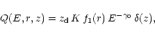
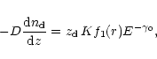
In general the propagation equation for CRs is described by
The main
conclusion was that almost all observations can be reasonably explained if
the halo extension is about several kpc, the injection spectrum of electrons
and protons Q(E) is a power-law (
![]() with
with
![]() -2.4), and the radially uniform velocity of advection
does not exceed the value of 20 kms-1. Compton scattering of relativistic
electrons was found to play a significant rôle in the halo
-2.4), and the radially uniform velocity of advection
does not exceed the value of 20 kms-1. Compton scattering of relativistic
electrons was found to play a significant rôle in the halo ![]() -ray
emission. However, this model failed to explain a smooth emissivity
distribution of
-ray
emission. However, this model failed to explain a smooth emissivity
distribution of ![]() -rays in the Galactic disk (see for details Dogiel
& Uryson 1988). Even in the case of a very extended halo with a radius
larger than 10 kpc the derived emissivity gradient (calculated for the
observed SN distribution) was larger than observed. Only for a
hypothetical uniform distribution of the sources in the disk the
calculations can reproduce the data.
-rays in the Galactic disk (see for details Dogiel
& Uryson 1988). Even in the case of a very extended halo with a radius
larger than 10 kpc the derived emissivity gradient (calculated for the
observed SN distribution) was larger than observed. Only for a
hypothetical uniform distribution of the sources in the disk the
calculations can reproduce the data.
This model was further developed by Bloemen et al. (1991, 1993). Extensive
investigations of the 3-dimensional diffusion-advection transport equation
for nucleons, low-energy electrons and the ![]() -rays showed that even in
the most favorable case of an extended halo with a vertical height as large
as 20 kpc, their model, although reproducing the COS B data marginally, is
not able to remove the signature of the observationally inferred SNR
source distribution, i.e. the distribution of the calculated
emissivity was still steeper than permitted by the data. The vertical
gradient of the advection velocity derived from the fluxes of stable and
radioactive nuclei near Earth had to be smaller than 15 kms-1/kpc. The other
unexpected conclusion was that the halo extension obtained from
the nuclear data was significantly less than estimated from the
-rays showed that even in
the most favorable case of an extended halo with a vertical height as large
as 20 kpc, their model, although reproducing the COS B data marginally, is
not able to remove the signature of the observationally inferred SNR
source distribution, i.e. the distribution of the calculated
emissivity was still steeper than permitted by the data. The vertical
gradient of the advection velocity derived from the fluxes of stable and
radioactive nuclei near Earth had to be smaller than 15 kms-1/kpc. The other
unexpected conclusion was that the halo extension obtained from
the nuclear data was significantly less than estimated from the ![]() -ray
data (see also Webber et al. 1992).
-ray
data (see also Webber et al. 1992).
A qualitative argument, how to populate the outer Galaxy with CRs, has been given by Erlykin et al. (1996) who invoke wind removal of particles in the inner Galaxy, combined with some return flow to the outer disk. It is hard to judge the merits of such a suggestion in the absence of any physics estimate. We therefore do not further consider such a possibility here.
Recently, Strong and collaborators in a series of papers (see Strong et al.
2000, and references therein) have developed a numerical method
for this model and made a new attempt to analyze the ![]() -ray emission
and the CR data, based on the latest data from COMPTEL, EGRET and OSSE.
They limited the analysis to radially uniform diffusion-advection and to
diffusion-reacceleration transport models, and concluded that no such
diffusion-advection model can adequately describe the data, in particular
the B/C ratio and the energy dependence. These authors claimed, however,
that by including reacceleration one can account for all the
observational data. A peculiar
consequence of their analysis was that they did not use the observed
supernova source distribution (see e.g., Kodeira 1974; Leahy & Xinji 1989;
Case & Bhattacharya 1996, 1998) as the input Q for Eq. (1), but
rather derived it from the
-ray emission
and the CR data, based on the latest data from COMPTEL, EGRET and OSSE.
They limited the analysis to radially uniform diffusion-advection and to
diffusion-reacceleration transport models, and concluded that no such
diffusion-advection model can adequately describe the data, in particular
the B/C ratio and the energy dependence. These authors claimed, however,
that by including reacceleration one can account for all the
observational data. A peculiar
consequence of their analysis was that they did not use the observed
supernova source distribution (see e.g., Kodeira 1974; Leahy & Xinji 1989;
Case & Bhattacharya 1996, 1998) as the input Q for Eq. (1), but
rather derived it from the ![]() -ray data to reproduce the observed
spatial variations of the emissivity in the disk. The result was a source
distribution that is flat in the radial direction.
-ray data to reproduce the observed
spatial variations of the emissivity in the disk. The result was a source
distribution that is flat in the radial direction.
Thus we see that the conventional model of unifrom diffusion-advection has
serious problems in spite of its evident achievements. One solution is to
assume that some of the observational data are not significant like the SN
distribution derived from the radio observations (Strong et al. 2000).
The alternative is to conclude that it is time to abandon the
standard model, which is what we do in this paper. We shall demonstrate,
that strong radial source gradients will be removed by a strong advection velocity in the halo (due to a Galactic wind driven by the CRs
themselves, see below) that varies with radius R and height z.
In addition anisotropic diffusion with different diffusion coefficients
![]() and
and ![]() in the disk and the halo, respectively, might also play a
rôle. It should be emphasized that a radially varying advection velocity
occurs naturally in spiral galaxies, even for a uniform source
distribution, because the gravitational potential increases towards the
centre, thus inducing stronger velocity gradients in this direction
(see Fig. 2), as has been shown by Breitschwerdt et al. (1991).
in the disk and the halo, respectively, might also play a
rôle. It should be emphasized that a radially varying advection velocity
occurs naturally in spiral galaxies, even for a uniform source
distribution, because the gravitational potential increases towards the
centre, thus inducing stronger velocity gradients in this direction
(see Fig. 2), as has been shown by Breitschwerdt et al. (1991).
The existence of strong advective CR transport in the Galactic halo has been shown on dynamical grounds in a number of papers in the past (Ipavich 1975; Breitschwerdt et al. 1987, 1991, 1993; Fichtner et al. 1991; Zirakashvili et al. 1996; Ptuskin et al. 1997). The key element of halo transport theory is that CRs, which by observations are known to escape from the Galaxy, resonantly generate waves by the so-called streaming instability (Kulsrud & Pearce 1969) leading to strong scattering of CRs. Therefore, even in the case of strong non-linear wave damping, advection is at least as important a CR transport mechanism out to large distances in the halo as diffusion, provided that the level of MHD-turbulence is high enough for coupling between CRs and MHD waves (Dogiel et al. 1994; Ptuskin et al. 1997). There is also growing indirect observational evidence of outflows from the interpretation of soft X-ray data of galactic halos in edge-on galaxies like NGC 4631 (Wang et al. 1995), and also of the soft X-ray background in our own Galaxy (Breitschwerdt & Schmutzler 1994, 1999). Furthermore, the near constancy of the spectral index of nonthermal radio continuum emission over large distances along the minor axis in the halo of edge-on galaxies is most naturally explained by an advective transport velocity of relativistic electrons (along with the nucleons) that is ever increasing with distance from the Galactic plane (Breitschwerdt 1994).
In the disk of spiral galaxies, the regular magnetic field is following
roughly the spiral arms and is therefore mostly parallel to the disk, with
noticeable deviations in some regions where outflow is expected.
Here, also a regular vertical component seems to be present (e.g. Hummel
et al. 1988),
which has been detected in a number of galaxies like NGC 4631,
NGC 5775 (Tüllman et al. 2000), and NGC 4217.
Multi-wavelength observations of the galaxy NGC 253 show a local
correlation between non-thermal radio continuum, H![]() and X-ray emission
near the disk-halo interface in off-nuclear regions (Dettmar 1992; M. Ehle,
private communication). This also spatially coincides with enhanced star
formation activity in the disk as can be seen from FIR data.
and X-ray emission
near the disk-halo interface in off-nuclear regions (Dettmar 1992; M. Ehle,
private communication). This also spatially coincides with enhanced star
formation activity in the disk as can be seen from FIR data.
Since the disk is not fully ionized in contrast to the halo and since waves are efficiently dissipated there by ion-neutral damping, the most important contribution to the random field in the disk is by turbulent mass motions, induced by supernova explosions and other stellar mass loss activity. Thus the wave spectrum will be very different from the one in the halo, where self-excited waves subject to nonlinear wave damping (Dogiel et al. 1994; Ptuskin et al. 1997), satisfying the gyro-resonance condition, dominate. Consequently, the averaged diffusion coefficient will be different in the Galactic disk and the halo (see Sect. 4). Therefore, we believe that anisotropic diffusion, together with radially varying advection, is the most general and most probable mode of CR transport to occur. We investigate the CR transport processes of diffusion and advection and discuss the possibility of flattening radial CR source gradients of a given SNR distribution (despite observational uncertainties) by particle propagation. In our view it is essential using the "natural'' boundary condition when calculating the response of CR transport to a given CR source distribution (whatever its observational limitations may be at the present time). This is in contrast to adjusting the source distribution a posteriori. To implement the transport processes properly we shall allow for radially varying advection, anisotropic diffusion, (different values of the diffusion coefficient parallel and perpendicular to the disk) and the appropriate boundary conditions to employ a cosmic ray distribution and then to calculate from these the resulting spatial distribution of CRs.
In Sect. 4 we discuss the question of anisotropic CR diffusion
and in Sect. 5 we introduce a simple model that describes
the observed CR source distribution. In the following
Sect. 6 we show heuristically (and in Sect. 8
also analytically) how a radially varying CR source distribution induces
variations in the CR energy density, which in turn leads to a radial
variation of the diffusion-advection boundary, ![]() ,
and the outflow
velocity, respectively, and thus to a tendency to flatten the radial
CR distribution and hence the
,
and the outflow
velocity, respectively, and thus to a tendency to flatten the radial
CR distribution and hence the ![]() -ray emissivity gradient. In
Sect. 7 we demonstrate by numerical calculations how such a
source distribution will naturally generate a radially varying outflow
velocity. In Sect. 8 we discuss in detail models of
different complexity for advective-diffusive transport with radially
varying outflow velocity, and show analytically how in each case for a
given CR source distribution its radial signature on the energetic
particle and
-ray emissivity gradient. In
Sect. 7 we demonstrate by numerical calculations how such a
source distribution will naturally generate a radially varying outflow
velocity. In Sect. 8 we discuss in detail models of
different complexity for advective-diffusive transport with radially
varying outflow velocity, and show analytically how in each case for a
given CR source distribution its radial signature on the energetic
particle and ![]() -ray distribution is reduced. The most advanced of
these models include
a dependence of galactic wind velocity on the CR source strength.
In addition a full analytic solution of the
3-dimensional diffusion-advection equation in axisymmetry for a given
realistic velocity dependence u(r,z), parallel and perpendicular to the
Galactic disk similar to the one derived in Sect. 7, is
calculated. In
Sect. 9 the source contributions to the "diffuse''
-ray distribution is reduced. The most advanced of
these models include
a dependence of galactic wind velocity on the CR source strength.
In addition a full analytic solution of the
3-dimensional diffusion-advection equation in axisymmetry for a given
realistic velocity dependence u(r,z), parallel and perpendicular to the
Galactic disk similar to the one derived in Sect. 7, is
calculated. In
Sect. 9 the source contributions to the "diffuse''
![]() -ray background at TeV energies are taken into account and shown
to be highly significant. This should allow an empirical test of our
theoretical picture. In Sect. 10 we discuss and summarize our
results. A number of detailed calculations can be found in the
Appendices A, B and C.
-ray background at TeV energies are taken into account and shown
to be highly significant. This should allow an empirical test of our
theoretical picture. In Sect. 10 we discuss and summarize our
results. A number of detailed calculations can be found in the
Appendices A, B and C.
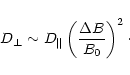
In most models of diffusive CR propagation, the diffusion tensor is
approximated by a scalar quantity D, representing spatially uniform
transport,
![]() ,
where
,
where
![]() -0.6 describes the energy dependence.
However, there are good reasons why the diffusion coefficient may be
anisotropic.
-0.6 describes the energy dependence.
However, there are good reasons why the diffusion coefficient may be
anisotropic.
The propagation of CRs in the interstellar medium is mainly determined by
their interaction with electric and magnetic fields. CRs interact strongly
with fluctuations of the magnetic field (MHD-waves) and are scattered
by them in pitch angle.
In the simplest case the total magnetic field consists of two components
and can be written as
| (2) |
Effective scattering of particles by these fluctuations occurs when the
interaction is resonant, i.e.
when the scale of the fluctuations in the magnetic field B0 is of the
order of the particle gyroradius.
This leads to a stochastic motion of particles through space;
the associated diffusion coefficient ![]() along
the magnetic field B0 is of the order of
along
the magnetic field B0 is of the order of
 |
(3) |
| (4) |
 |
(6) |
The situation is more complex if there exists also a large scale random
magnetic field ![]() whose scale is much larger than the particle gyroradius:
whose scale is much larger than the particle gyroradius:
| (7) |
The procedure to derive the transport equation for CRs in this case was
described, e.g. by Toptygin (1985), who showed that the maximum value of
![]() is:
is:
 |
(8) |
A more precise analysis (see Berezinsky et al. 1990, Chap. 9) shows,
however, that in the interstellar medium the correlation between the
components of the diffusion tensor leads to an effective perpendicular
diffusion coefficient:
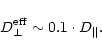 |
(9) |
The inference on the spatial distribution of CR sources from direct observations is plagued by a number of problems. From energy requirements for the bulk of CRs below 1015 eV, it is known that the only non-hypothetical Galactic candidates for the sources are SNRs and pulsars, with global energetic requirements favouring the former. SNRs can be best studied in the radio continuum and in soft X-rays, but as low surface brightness objects larger and older remnants are systematically missed. Since samples are usually flux limited, the more distant objects will be lost as well. Pulsars on the other hand should be present in the Galaxy in large numbers. However they are only detectable if their narrow beams happen to cross the line of sight of the observer or, in X-rays, as isolated old neutron stars; so far only four candidates are known from the ROSAT All-Sky Survey (Neuhäuser & Trümper 1999). Therefore selection effects will bias samples heavily in both cases.
Based on the observations of SNRs by Kodeira (1974) and pulsars by
Seiradakis (1976), Stecker & Jones (1977) have
given a simple radial
Galactic distribution of the form
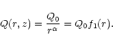
To determine the proportionality constant q0 for the distribution
given in Eq. (10), we use the results obtained by Leahy & Xinji (1989)
who used the catalogue of Li (1985) derived from radio observations.
Leahy & Xinji (1989) considered shell-type SNRs and applied empirical
correction factors due to the incompleteness of the flux limited sample.
The spatial distribution thus obtained shows a peak at 4-6 kpc from the
Galactic center (see Fig. 1), assuming an overall rotational symmetry.
A more systematic study has recently been undertaken
by Case & Bhattacharya (1998), who have made a careful analysis of an
enhanced Galactic SNR sample, using an improved ![]() relation.
These authors
find a peak in the distribution at around 5 kpc
relation.
These authors
find a peak in the distribution at around 5 kpc![]() and a scale length of
and a scale length of ![]() 7 kpc, thus confirming the gross features of the older work.
The number of SNRs in an annulus of width dx is given by
7 kpc, thus confirming the gross features of the older work.
The number of SNRs in an annulus of width dx is given by
On the other hand, the total number of SNRs that should be observable at
present is their production rate ![]() times their average life
time
times their average life
time
![]() before they merge with the hot intercloud medium and
lose their individual appearance, or observationally escape the
detection limit. The rate at which SNe occur in the disk
is
before they merge with the hot intercloud medium and
lose their individual appearance, or observationally escape the
detection limit. The rate at which SNe occur in the disk
is
![]() per century for randomly exploding stars (van den
Bergh 1990, 1991) and 0.45 per century
for explosions occurring in OB associations (Evans et al. 1989),
giving a total SN rate in the Milky Way disk of
per century for randomly exploding stars (van den
Bergh 1990, 1991) and 0.45 per century
for explosions occurring in OB associations (Evans et al. 1989),
giving a total SN rate in the Milky Way disk of
![]() per century.
The total number of SNRs in the disk is then given by
per century.
The total number of SNRs in the disk is then given by
Dragicevich et al. (1999) have analyzed also the radial distribution of
SNe in a sample of 218
external galaxies of different Hubble types, corrected for inclination
angle. The data were sorted into radial bins and the numbers converted into
SNe surface densities.
They showed that the radial SN surface distribution can be well fitted by an
exponential radial decrease of the form
 |
(15) |
![\begin{figure}
\par\includegraphics[width=8.8cm,clip]{h2935F1.eps} \end{figure}](/articles/aa/full/2002/13/aah2935/img91.gif) |
Figure 1:
Surface density of SNRs and supernovae, respectively,
in galaxies as a function
of Galactocentric distance R. The solid curve, Q(R), gives
a fit to the SNR distribution of the Milky Way and is given by
|
| Open with DEXTER | |
More specifically, we
consider SNRs as the primary sources for the Galactic CRs. Each remnant
results from an energy deposition of
![]() ,
which is converted into relativistic particles with a certain efficiency
,
which is converted into relativistic particles with a certain efficiency
![]() -0.5 (Drury et al. 1989; Berezkho & Völk 2000);
the individual value of
-0.5 (Drury et al. 1989; Berezkho & Völk 2000);
the individual value of ![]() is poorly known from theory due to
uncertainties in the injection process and depends e.g., on the value and
orientation of the circumstellar magnetic field.
SNe exploding inside a superbubble, i.e. a hot tenuous medium, initially
generate low
Mach number shocks, which are less efficient in accelerating particles.
After a time of the order of the sound crossing time, however, the shock
impinges on the much colder and denser surrounding shell and becomes progressively
stronger thereby accelerating particles more efficiently; this should
to lowest
order compensate for the initially decreased efficiency in the hot ambient
medium. We would expect that
due to the continuous energy input by successive SN explosions
also a long lived shock would be able to accelerate particles to energies
in excess of 1014 eV, albeit adiabatic energy losses
would become more and more severe with time. Since the diffusion coefficient of CRs
increases with energy, advective transport of particles significantly above
1 GeV will be the dominant mode of transport only at larger distances from
the Galactic plane. Therefore these particles will quickly fill an
extended halo and not generate many
is poorly known from theory due to
uncertainties in the injection process and depends e.g., on the value and
orientation of the circumstellar magnetic field.
SNe exploding inside a superbubble, i.e. a hot tenuous medium, initially
generate low
Mach number shocks, which are less efficient in accelerating particles.
After a time of the order of the sound crossing time, however, the shock
impinges on the much colder and denser surrounding shell and becomes progressively
stronger thereby accelerating particles more efficiently; this should
to lowest
order compensate for the initially decreased efficiency in the hot ambient
medium. We would expect that
due to the continuous energy input by successive SN explosions
also a long lived shock would be able to accelerate particles to energies
in excess of 1014 eV, albeit adiabatic energy losses
would become more and more severe with time. Since the diffusion coefficient of CRs
increases with energy, advective transport of particles significantly above
1 GeV will be the dominant mode of transport only at larger distances from
the Galactic plane. Therefore these particles will quickly fill an
extended halo and not generate many ![]() -rays in the disk via
-rays in the disk via ![]() -decay.
-decay.
Bykov & Fleishman (1992) have argued that successive explosions inside
a bubble can generate strong turbulence, which should transform a
significant amount of the total free energy to cosmic rays. However,
at the same time the injection rate at the shocks may be reduced as a
result of shock modification due to previously generated CR particles.
With the details of the acceleration mechanism in superbubbles being
still debatable, we believe that
to lowest order there is no difference in the overall energy transfer from
thermal plasma to CRs, if a SN explodes inside a superbubble or just forms a
single remnant. Thus the energy production rate of CRs should be roughly
proportional to the number of SN explosions, regardless whether they
occur in the general ISM or inside a superbubble.
The numerical difference in the derived CR energy density (and CR pressure)
(cf. Eqs. (18) and (17)), however, between treating particle
acceleration in superbubbles as equal to single remnants, and disregarding
acceleration in superbubbles altogether, is small.
According to the previous section it amounts to a factor
![]() ,
and is therefore well
below the uncertainty in the acceleration efficiency
,
and is therefore well
below the uncertainty in the acceleration efficiency ![]() .
In the following, we tend to be conservative and retain a low value of
.
In the following, we tend to be conservative and retain a low value of
![]() .
.
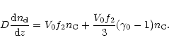
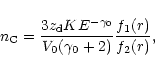
Using the results from Sect. 5 we can estimate the local
number of
SNRs within a circular ring of the Galaxy with a width of, say, 2 kpc.
Relating the SN rate directly to the number of observable SNRs by
Eq. (14) and writing (cf. Eq. (11))
The diffuse ![]() -ray intensity resulting from
-ray intensity resulting from ![]() -decay photons is
-decay photons is
In order to obtain
![]() for a weak
for a weak ![]() -ray gradient,
we should assume that
-ray gradient,
we should assume that
 |
(26) |
As we have deduced in the last section, the CR pressure
![]() in
the disk is a
radially dependent quantity, and therefore we expect the outflow
velocity, u(x), and the mass loss rate,
in
the disk is a
radially dependent quantity, and therefore we expect the outflow
velocity, u(x), and the mass loss rate, ![]() ,
to be also radially
dependent. In an earlier paper (Breitschwerdt et al. 1991) we have
shown that such a behaviour already exists as a consequence of the radial
dependence of the gravitational potential. The net result was a monotonic
decrease (increase) of terminal velocity (mass loss rate) with increasing
Galactic radius for a radially constant mass density,
,
to be also radially
dependent. In an earlier paper (Breitschwerdt et al. 1991) we have
shown that such a behaviour already exists as a consequence of the radial
dependence of the gravitational potential. The net result was a monotonic
decrease (increase) of terminal velocity (mass loss rate) with increasing
Galactic radius for a radially constant mass density, ![]() .
Now we have superposed the radial variation of the CR source
density Q1(x) and investigate in the following how this changes
the outflow.
However, Eq. (21) is an implicit equation, since
.
Now we have superposed the radial variation of the CR source
density Q1(x) and investigate in the following how this changes
the outflow.
However, Eq. (21) is an implicit equation, since
![]() depends
on
depends
on
![]() ,
which in turn depends on the energy
density available in CRs, i.e.
,
which in turn depends on the energy
density available in CRs, i.e.
![]() and thus
and thus
![]() itself, to drive the outflow.
To that end we have performed self-consistent galactic wind
calculations of the fully nonlinear equations, in which for a given
gravitational potential of the Milky Way,
and a relativistic CR gas (
itself, to drive the outflow.
To that end we have performed self-consistent galactic wind
calculations of the fully nonlinear equations, in which for a given
gravitational potential of the Milky Way,
and a relativistic CR gas (
![]() ),
together with a spatially averaged mass density
),
together with a spatially averaged mass density
![]() ,
an average thermal
pressure
,
an average thermal
pressure
![]() ,
an averaged halo magnetic field
,
an averaged halo magnetic field
![]() ,
and a small average level of wave amplitude
,
and a small average level of wave amplitude
![]() ,
the advection-diffusion boundary
,
the advection-diffusion boundary
![]() ,
,
![]() and
and
![]() are calculated
self-consistently, using
q0 = 1492, the value derived from the numerical
integration of Eq. (12) (see Sect. 5).
The form of the potential (including, disk, bulge and dark matter halo) and
the opening of the flux tube due to geometrical divergence are the same as
used by Breitschwerdt et al. (1991).
are calculated
self-consistently, using
q0 = 1492, the value derived from the numerical
integration of Eq. (12) (see Sect. 5).
The form of the potential (including, disk, bulge and dark matter halo) and
the opening of the flux tube due to geometrical divergence are the same as
used by Breitschwerdt et al. (1991).
![\begin{figure}
\par\includegraphics[width=8.8cm,clip]{h2935F2.eps} \end{figure}](/articles/aa/full/2002/13/aah2935/img142.gif) |
Figure 2:
Escape speed,
|
| Open with DEXTER | |
![\begin{figure}
\par\includegraphics[angle=-90,width=8.8cm,clip]{h2935F3.ps} \end{figure}](/articles/aa/full/2002/13/aah2935/img143.gif) |
Figure 3:
Dependence of the diffusion-advection boundary,
|
| Open with DEXTER | |
It can be seen from comparison of
![]() and
and
![]() ,
as obtained from the fully nonlinear calculations, that the simple
ansatz of Eq. (19) is indeed fulfilled. The functional dependence
of
,
as obtained from the fully nonlinear calculations, that the simple
ansatz of Eq. (19) is indeed fulfilled. The functional dependence
of
![]() with radius is straightforward to understand. Close to the
Galactic centre, the gravitational pull is strongest, as can be seen from
with radius is straightforward to understand. Close to the
Galactic centre, the gravitational pull is strongest, as can be seen from
![]() in Fig. 2; since we chose all other quantities
being the same across the disk (constant density, thermal pressure,
magnetic field strength), the outflow velocity, and hence mass loss rate,
are smallest here. Equation (19) then tells us, that
in Fig. 2; since we chose all other quantities
being the same across the disk (constant density, thermal pressure,
magnetic field strength), the outflow velocity, and hence mass loss rate,
are smallest here. Equation (19) then tells us, that
![]() must
be largest. At the outer parts of the Galaxy, the gravitational field
becomes weaker, but also the source distribution, and hence the CR pressure,
decrease exponentially, and so the outflow velocity (cf. Fig. 2)
also decreases, and
must
be largest. At the outer parts of the Galaxy, the gravitational field
becomes weaker, but also the source distribution, and hence the CR pressure,
decrease exponentially, and so the outflow velocity (cf. Fig. 2)
also decreases, and
![]() must increase again (see Fig. 3).
It is noteworthy that
the maximum of
must increase again (see Fig. 3).
It is noteworthy that
the maximum of
![]() and the minimum of
and the minimum of
![]() at
at
![]() kpc do not coincide with the maximum of Q1(r) and
kpc do not coincide with the maximum of Q1(r) and
![]() ,
respectively, at
,
respectively, at
![]() kpc. This must be a consequence
of the interplay between the gravitational field
and the source distribution in the fully nonlinear equations (cf.
Breitschwerdt et al. 1991).
kpc. This must be a consequence
of the interplay between the gravitational field
and the source distribution in the fully nonlinear equations (cf.
Breitschwerdt et al. 1991).
Finally we mention that the choice of constant boundary conditions across
the Galactic disk is a conservative one. In reality we should also enhance
the thermal temperature and pressure in regions of higher supernova activity.
The net effect would be a more pronounced peak in outflow velocity and
a deeper minimum in
![]() ,
respectively, and therefore an even "better''
quantitative proportionality between
,
respectively, and therefore an even "better''
quantitative proportionality between
![]() and
Q1(r) according to Eq. (24).
and
Q1(r) according to Eq. (24).
In the following we discuss several advection models
(some including also anisotropic spatial diffusion), in which
we examine in detail the ideas presented in Sect. 6. We show that
for a given radial CR source distribution function
![]() ,
we can find a function
,
we can find a function
![]() ,
for which the effect of the
radially varying Galactic wind velocity leads to an almost uniform CR
distribution in
the disk. We refer to relations
f2(r) = F(f1(r)) as "compensation
equations''. It is thus possible to explain the observational data
by pure CR propagation effects.
,
for which the effect of the
radially varying Galactic wind velocity leads to an almost uniform CR
distribution in
the disk. We refer to relations
f2(r) = F(f1(r)) as "compensation
equations''. It is thus possible to explain the observational data
by pure CR propagation effects.
To fix ideas, we start out with a functional relation for the Galactic CR
source distribution of the form
We start from the simplest one-dimensional CR transport model, which is an extreme case of anisotropic diffusion, since only propagation in the z-direction is allowed. In this case the galactocentric radius r is simply a parameter in the model.
The one-dimensional diffusion-advection equation for CR nucleons can be
written as
 |
(30) |
The boundary conditions for CRs are determined either by free escape
into intergalactic space, if the density of electromagnetic fluctuations
generated by the CR flux decreases fast enough (see Dogiel et al. 1994), or
by CR advection in a galactic wind to infinity (Breitschwerdt et al. 1991; Ptuskin et al. 1997), if the level of fluctuations is high
enough.
Which of these cases is relevant for the Galaxy, is the subject of a
separate investigation. Fortunately, CR spectra and densities in
the disk are independent of the boundary conditions far away from the
Galactic plane, if there is an outer region of advective transport.
In the case we discuss here, it is assumed that the CR propagation region can
be formally divided into a diffusion
halo wrapping around the Galactic plane and an adjacent advection region,
reaching out to intergalactic space.
These two regions are separated by a boundary surface, ![]() ,
at which both the
CR density and the flux have to be continuous.
The sources are concentrated in the disk
and are supposed to emit a power-law spectrum of particles
,
at which both the
CR density and the flux have to be continuous.
The sources are concentrated in the disk
and are supposed to emit a power-law spectrum of particles
 |
(31) |
The location of the transition boundary
for a constant diffusion coefficient D and advection velocity V0 is
determined in this approximation by
 |
(32) |
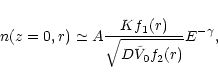
| (35) |
| (36) |
 |
(37) |
 |
(38) |
 |
(39) |
 |
(41) |
| f1(r) = f2(r) , | (42) |
From Eq. (40) we can also estimate the total pressure, ![]() ,
of CRs in the disk, which is
,
of CRs in the disk, which is
 |
(45) |
 |
(46) |
Based on the conclusions of the previous sections, we can generalize the
one-dimensional solution obtained by Bloemen
et al. (1993), taking into account radial variations of the sources and
the wind velocity. Let us suppose that the advection velocity has the form
 |
(48) |
 |
(49) |
We find that a vanishing radial dependence of the CR distribution,
![]() ,
can be obtained if
,
can be obtained if
| f12(r) = f2(r). | (50) |
These simple analytical solutions of the one-dimensional transport
equation show that the main effect, which formally leads to the
"compensation", is a curved transition boundary between diffusion and
advection regions, i.e.
 |
(51) |
In the framework of the pure one-dimensional model it is unimportant
how far from the Galactic plane the
boundary
![]() is, but as we shall see, this figure will be essential
for the three-dimensional case.
is, but as we shall see, this figure will be essential
for the three-dimensional case.
To demonstrate the effect of radial changes of the boundary
![]() between
regions of diffusive and advective propagation of CRs, we
investigate the diffusion-advection equation with a given radial dependence
of the wind velocity and the source density in a more realistic cylindrical
geometry (axial symmetry, i.e.
between
regions of diffusive and advective propagation of CRs, we
investigate the diffusion-advection equation with a given radial dependence
of the wind velocity and the source density in a more realistic cylindrical
geometry (axial symmetry, i.e.
![]() )
with the
velocity varying as
)
with the
velocity varying as
 |
(53) |
Equation (54) can be solved analytically
if we restrict ourselves to self-similar solutions, in which
the distribution function does not vary with r and z independently.
The price we have to pay is that there is no unique solution that
covers both
![]() and
and
![]() .
Instead
a similarity solution is found for
.
Instead
a similarity solution is found for ![]() and r>0, and
one for z>0, which have to match in overlapping
regions. We start out with the latter one, applying a
transformation of independent variables of the form
and r>0, and
one for z>0, which have to match in overlapping
regions. We start out with the latter one, applying a
transformation of independent variables of the form
| b1 | = | ||
| b4 | = | (59) |
We can derive an analytical solution of this equation in the form (see
Bakhareva & Smirnova 1980)
 |
(60) |
The unknown coefficients ![]() ,
C and A are determined from the system
of algebraic equations which one can obtain from Eq. (58)
by equating the
coefficients for the different powers of
,
C and A are determined from the system
of algebraic equations which one can obtain from Eq. (58)
by equating the
coefficients for the different powers of ![]() to zero. The resulting system
of algebraic equations is given by
to zero. The resulting system
of algebraic equations is given by
| A b1+b4=0 | (61) |
| 2C (1+b1)+A (A+b2)+b5=0 | (62) |
| 2C (2A+b2)-A (2-b3) + b4=0 | (63) |
| 2C (2C-1+b3)+ b5=0. | (64) |
From the system of Eqs. (61)-(64) it can be
deduced that
| A | = | (65) | |
| C | = | (66) | |
| = | 0 , | (67) | |
| = | -1 . | (68) |
 |
(69) |
The limit
![]() corresponds to
corresponds to ![]() so that
so that
| = | |||
| = | (70) |
The full solution of Eq. (54) reads
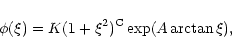
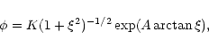
In order to study the radial behaviour of the distribution function near
z=0 a different self-similar ansatz is used, which can be extended down
to the spatial region near the sources.
The similarity variable has the form
 |
(79) |
 |
(81) |
 |
(84) |
From the asymptotic expansion of hypergeometrical functions at
![]() ,
we find that the solution Eq. (82) depends on
,
we find that the solution Eq. (82) depends on ![]() as
as
 |
(86) |
| (87) |
 |
(88) |
 |
(89) |
 |
(90) |
Since close to the sources,
![]() ,
,
![]() ,
we derive
from Eq. (75)
,
we derive
from Eq. (75)
 |
(91) |
 |
(92) |
 |
(93) |
| f22=f1 . | (94) |
![\begin{figure}
\par\includegraphics[width=8.8cm,clip]{h2935F4.eps} \end{figure}](/articles/aa/full/2002/13/aah2935/img267.gif) |
Figure 4:
The nucleon distribution function n(r,z) is plotted in
arbitrary units as a function of Galactocentric radius r and
height z above the plane. The radial and vertical diffusion
coefficients are
|
| Open with DEXTER | |
![\begin{figure}
\par\includegraphics[width=8.8cm,clip]{h2935F5.eps} \end{figure}](/articles/aa/full/2002/13/aah2935/img268.gif) |
Figure 5:
Same as Fig. 4, but the radial and vertical diffusion
coefficients are now different, viz.
|
| Open with DEXTER | |
![\begin{figure}
\par\includegraphics[width=8.8cm,clip]{h2935F6.eps} \end{figure}](/articles/aa/full/2002/13/aah2935/img271.gif) |
Figure 6:
Same as Fig. 5, with
|
| Open with DEXTER | |
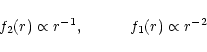
Moreover, according to Fig. 5, a stronger radial than vertical mixing
of CRs due to anisotropic diffusion leads to a further flattening of the
nucleon distribution function and hence to a weaker diffuse ![]() -ray
gradient. We expect this to happen in the Galactic disk, where the
geometry of the large scale magnetic field is mainly parallel to the disk.
In contrast, in the halo a substantial vertical
-ray
gradient. We expect this to happen in the Galactic disk, where the
geometry of the large scale magnetic field is mainly parallel to the disk.
In contrast, in the halo a substantial vertical ![]() -component
might exist (like e.g. in NGC 4631), resulting in a larger value
of
-component
might exist (like e.g. in NGC 4631), resulting in a larger value
of ![]() as compared to
as compared to
![]() .
As can be seen from Fig. 6 this
effect is competing to some extent with the also vertically directed
advection velocity, and therefore the distribution function is similar to
the one shown in Fig. 4.
.
As can be seen from Fig. 6 this
effect is competing to some extent with the also vertically directed
advection velocity, and therefore the distribution function is similar to
the one shown in Fig. 4.
In summary we conclude that the value of the halo extension calculated from the gradient data in the framework of the isotropic diffusion model may indeed be an artifact. In the next section we outline a general solution.
We now want to work out a general solution of the stationary two-dimensional
CR transport equation for nucleons, without any restriction of the radial
behavior of the source distribution Q(r,z). In the following we use
N(r, z, E) for the nucleon distribution function in order to avoid
confusion with the number n for the enumeration of the poles in our
solutions.
 |
(96) |
We are not so much interested in energy dependent than spatially anisotropic
diffusion and advection, and so, for convenience, we set ![]() .
For the nucleon component other than adiabatic losses are negligible
(dE/dt=0); thus Eq. (94) in axial symmetry reads
.
For the nucleon component other than adiabatic losses are negligible
(dE/dt=0); thus Eq. (94) in axial symmetry reads
| Q1(r) = Q0 f1(r) , | (98) |
![\begin{figure}
\par\includegraphics[angle=-90,width=8.8cm,clip]{h2935F7.eps} \end{figure}](/articles/aa/full/2002/13/aah2935/img285.gif) |
Figure 7:
Galactic wind outflow velocity (z-component),
|
| Open with DEXTER | |
It is clear from Eq. (96) that the effect of anisotropic
diffusion corresponds to stretching or compressing scales in respective
directions, since in the new variables,
![]() ,
and,
,
and,
![]() ,
we recover the equation for isotropic diffusion. Obviously, this
may also change the gradient of the cosmic ray density in the disk, but we will
show that rather strong modifications of the density (including the observed
uniform distribution of cosmic rays) can be obtained for spatially nonuniform
advection.
,
we recover the equation for isotropic diffusion. Obviously, this
may also change the gradient of the cosmic ray density in the disk, but we will
show that rather strong modifications of the density (including the observed
uniform distribution of cosmic rays) can be obtained for spatially nonuniform
advection.
In order to solve Eq. (96) analytically, we apply the following
transformations
| x | = | (122) | |
| = | (123) |
 |
(124) |
Thus the solution of the homogeneous equation reads
Applying the linear transformation
| = | |||
| (131) |
We now return to the inhomogeneous equation (Eq. (119)).
For
![]() ,
Eq. (131) is a valid solution; in order
to evaluate the solution at
,
Eq. (131) is a valid solution; in order
to evaluate the solution at ![]() we integrate Eq. (119)
in the infinitesimal range
we integrate Eq. (119)
in the infinitesimal range
![]() ,
with
,
with
![]() and then take the limit
and then take the limit
![]() .
.
Exploiting the properties of the solution ![]() outlined above, and
noting that the integration over an odd function vanishes, we obtain
after a little algebra
outlined above, and
noting that the integration over an odd function vanishes, we obtain
after a little algebra
Manipulating the ![]() -functions with help of the relations
in Appendix B (B.7-B.9) the solution for
-functions with help of the relations
in Appendix B (B.7-B.9) the solution for
![]() reads
reads
Using the solution for ![]() we can now, as a special case, calculate
the full solution in the disk, i.e.
N(r, z=0,E)).
The Green's function is then given by Eq. (117)
we can now, as a special case, calculate
the full solution in the disk, i.e.
N(r, z=0,E)).
The Green's function is then given by Eq. (117)
Let K = i k, we obtain
![\begin{displaymath}G(0;\varrho,
\varrho^{\prime}) = -\frac{i}{2 \pi} \int_{-i \i...
...t[-K\left(\varrho - \varrho^{\prime}\right)\right] {\rm d}K ,
\end{displaymath}](/articles/aa/full/2002/13/aah2935/img362.gif) |
(138) |
 | (142) | ||
 | (143) | ||
 |
|||
 |
|||
 |
|||
 |
(144) | ||
| = | (145) |
Then we get from the theorem of residues (the residues of Gamma functions
![]() at
n=0,-1,-2,... are given by
at
n=0,-1,-2,... are given by
![]() )
)
| = | (147) | ||
| = | (148) | ||
| Kn | = | (149) | |
| = | (150) |
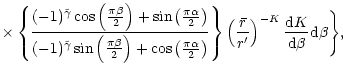
Inside the source region (![]() ), N(r) can be
written as
), N(r) can be
written as
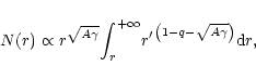 |
(151) |
 |
(152) |
In the diffusion dominated case (![]() )
the values of the integrals are
determined by the source
distribution. Here we should take into account the integral over
)
the values of the integrals are
determined by the source
distribution. Here we should take into account the integral over ![]() ,
which is not zero (see Appendix C).
Far away from the disk, i.e.
,
which is not zero (see Appendix C).
Far away from the disk, i.e. ![]() ,
the distribution function is
determined
by the only pole,
,
the distribution function is
determined
by the only pole, ![]() ,
which is inside the contour
,
which is inside the contour ![]() (see
Fig. C.5). Therefore independent of the source distribution, we have
(see
Fig. C.5). Therefore independent of the source distribution, we have
 |
(153) |
Therefore we conclude from these analyses that a more or less uniform CR
distribution in the disk can be expected, if advection is strong,
i.e. ![]() .
.
The "compensation'' equation in this case reads
| f2(r)=f1(r) . | (154) |
The examples of the last section substantiate our argument that transport
effects should be responsible for all but eliminating the ![]() -ray
gradient in the GeV energy range. This ignores possible contributions to
the
-ray
gradient in the GeV energy range. This ignores possible contributions to
the ![]() -ray flux from the sources themselves. In fact, SNRs as CR
sources are expected to accumulate the accelerated CRs before
releasing them into the ISM at the end of their lifetime. In nuclear
collisions with thermal gas atoms or (for electrons) with photons inside
the remnant, this high density of energetic particles will produce a
strong
-ray flux from the sources themselves. In fact, SNRs as CR
sources are expected to accumulate the accelerated CRs before
releasing them into the ISM at the end of their lifetime. In nuclear
collisions with thermal gas atoms or (for electrons) with photons inside
the remnant, this high density of energetic particles will produce a
strong ![]() -ray intensity that contributes a "diffuse'' background if
these sources are unresolved. In fact the ensemble of Galactic SNRs,
expected to be strongly concentrated in the disk, will constitute such a
background with typically less than about 10 such sources along a line of
sight in the disk. They will be unresolved in GeV
-ray intensity that contributes a "diffuse'' background if
these sources are unresolved. In fact the ensemble of Galactic SNRs,
expected to be strongly concentrated in the disk, will constitute such a
background with typically less than about 10 such sources along a line of
sight in the disk. They will be unresolved in GeV ![]() -rays, except for
a few well-known nearby objects (Berezhko & Völk 2000); also their
collective flux contributes less than 10% to the overall
-rays, except for
a few well-known nearby objects (Berezhko & Völk 2000); also their
collective flux contributes less than 10% to the overall ![]() -ray
flux. However, we know that the CR source spectrum is much harder
-ray
flux. However, we know that the CR source spectrum is much harder
![]() than the diffuse Galactic CR energy spectrum
(
than the diffuse Galactic CR energy spectrum
(
![]() ), and therefore the source contribution will equal the truly
diffuse
), and therefore the source contribution will equal the truly
diffuse ![]() -ray flux at about 100 GeV and become even dominant at
about 103 GeV (= 1 TeV).
-ray flux at about 100 GeV and become even dominant at
about 103 GeV (= 1 TeV).
If the sources collectively dominate in the form of an unresolved
"diffuse'' background at very high ![]() -ray energies, then it should
be possible to observe the average CR source distribution and even the
average CR source spectrum (!) along the Galactic disk in the TeV range.
Present observations at TeV energies have not yet been able to detect this
"diffuse'' background. However, the experimental upper limits and the
predicted "diffuse'' flux are so close to each other (Aharonian et al.
2001) that an instrumental increase by an order of magnitude should lead
to a detection. The next generation of TeV instruments like H.E.S.S.,
CANGAROO, MAGIC or Veritas, that has this sensitivity, will come on line soon.
The comparison of such a detected TeV-distribution with the radial shape
of the source distribution from radio studies would constitute a stringent
empirical test on our theoretical arguments about the transport effects on
the truly diffuse Galactic CR component. It also shows the basic
importance of
-ray energies, then it should
be possible to observe the average CR source distribution and even the
average CR source spectrum (!) along the Galactic disk in the TeV range.
Present observations at TeV energies have not yet been able to detect this
"diffuse'' background. However, the experimental upper limits and the
predicted "diffuse'' flux are so close to each other (Aharonian et al.
2001) that an instrumental increase by an order of magnitude should lead
to a detection. The next generation of TeV instruments like H.E.S.S.,
CANGAROO, MAGIC or Veritas, that has this sensitivity, will come on line soon.
The comparison of such a detected TeV-distribution with the radial shape
of the source distribution from radio studies would constitute a stringent
empirical test on our theoretical arguments about the transport effects on
the truly diffuse Galactic CR component. It also shows the basic
importance of ![]() -ray surveys over a large range in energies and
radial distance.
-ray surveys over a large range in energies and
radial distance.
It is common practice to determine from the intensities of different
CR components near Earth the average
diffusion coefficient in the Galaxy, the velocity of advection, the
height of the CR halo in the direction perpendicular to the Galactic plane,
and the CR injection spectrum, just to name the most important ones.
Based on this hypothesis the nearly uniform radial
CR distribution, derived from the measurement of diffuse Galactic
![]() -rays, can be reproduced only
if there exists thorough spatial mixing of CRs in the framework of an extended
halo (if CR diffusion is isotropic). Hence in such a case local and
global properties of CRs do not differ from each other.
However, the inferred halo height from chemical composition
(
-rays, can be reproduced only
if there exists thorough spatial mixing of CRs in the framework of an extended
halo (if CR diffusion is isotropic). Hence in such a case local and
global properties of CRs do not differ from each other.
However, the inferred halo height from chemical composition
(
![]() kpc; see e.g., Bloemen et al. 1991, 1993; Webber et al. 1993;
Lukasiak et al. 1994) is clearly inconsistent with the value derived from
the interpretation of the
kpc; see e.g., Bloemen et al. 1991, 1993; Webber et al. 1993;
Lukasiak et al. 1994) is clearly inconsistent with the value derived from
the interpretation of the ![]() -ray data (
-ray data (
![]() kpc; cf. Dogiel
& Uryson 1988; Bloemen et al. 1993)
within the framework of an isotropic diffusion model (see Appendix A).
We therefore conclude that the halo size derived
from CR nuclear data reflects only a local value near Earth, and
the huge halo extension derived previously from
kpc; cf. Dogiel
& Uryson 1988; Bloemen et al. 1993)
within the framework of an isotropic diffusion model (see Appendix A).
We therefore conclude that the halo size derived
from CR nuclear data reflects only a local value near Earth, and
the huge halo extension derived previously from ![]() -ray data may be an
artifact, since it relies on the validity of global values for locally obtained
CR data. This conclusion is supported by our numerical galactic wind
simulations, which show that the vertical distance of the diffusion-advection
transition boundary from the Galactic plane, is inversely proportional to
the CR source power and not spatially constant as been previously assumed.
Radio observations of external galaxies indicate a large-scale magnetic field
geometry, which is mainly parallel to the major axis in the disk, and if
a halo field exists, it is parallel to the minor axis.
Therefore we expect that CR diffusion is in general anisotropic, with
a radial diffusion coefficient
-ray data may be an
artifact, since it relies on the validity of global values for locally obtained
CR data. This conclusion is supported by our numerical galactic wind
simulations, which show that the vertical distance of the diffusion-advection
transition boundary from the Galactic plane, is inversely proportional to
the CR source power and not spatially constant as been previously assumed.
Radio observations of external galaxies indicate a large-scale magnetic field
geometry, which is mainly parallel to the major axis in the disk, and if
a halo field exists, it is parallel to the minor axis.
Therefore we expect that CR diffusion is in general anisotropic, with
a radial diffusion coefficient
![]() in the disk, which is much
larger than diffusion in the perpendicular direction,
in the disk, which is much
larger than diffusion in the perpendicular direction, ![]() ,
and vice versa
in the halo. In this case the initially inhomogeneous CR
distribution, due to a radially varying source distribution in the disk, is
smeared out, whereas in the halo the dominant diffusion component
,
and vice versa
in the halo. In this case the initially inhomogeneous CR
distribution, due to a radially varying source distribution in the disk, is
smeared out, whereas in the halo the dominant diffusion component ![]() can be superposed by a strong advection velocity, which may determine
the spatial particle distribution.
can be superposed by a strong advection velocity, which may determine
the spatial particle distribution.
It would be desirable to have a high enough spatial resolution and
photon statistics in the future to observe the radial distribution
of diffuse ![]() -rays above 100 MeV in nearby edge-on galaxies,
such as NGC 253. However, it seems unlikely that both space-borne and
ground-based
-rays above 100 MeV in nearby edge-on galaxies,
such as NGC 253. However, it seems unlikely that both space-borne and
ground-based ![]() -ray observatories will satisfy this requirement
in the near future. Thus the only direct observation of the CR source
distribution in the Galaxy will be possible with next generation
TeV instruments like H.E.S.S.
-ray observatories will satisfy this requirement
in the near future. Thus the only direct observation of the CR source
distribution in the Galaxy will be possible with next generation
TeV instruments like H.E.S.S.
Acknowledgements
DB acknowledges support from the Deutsche Forschungsgemeinschaft (DFG) by a Heisenberg fellowship. He thanks the Max-Planck-Institut für Kernphysik in Heidelberg, the Max-Planck-Institut für extraterrestrische Physik in Garching, and the Department of Astrophysical Sciences of Princeton University, where this research has been carried out, for support and hospitality. DB thanks Russell Kulsrud for many interesting discussions.
VAD acknowledges financial support from the Alexander von Humboldt-Stiftung which was very essential for these collaborative researches. This work was prepared during his visit to Max-Planck-Institut für extraterrestrische Physik (Garching) and he is grateful to his colleagues from this institute for helpful and fruitful discussions. The final version of the paper was partly done at the Institute of Space and Astronautical Science. VAD thanks his colleagues from the institute and especially Prof. H. Inoue for their warm hospitality.
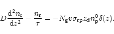
For a one-dimensional
diffusion model the system of equations for the density of stable, ![]() ,
and
radioactive,
,
and
radioactive, ![]() ,
nuclei is given by
,
nuclei is given by
 |
(A.1) |
 |
(A.2) |
| (A.3) |
Here z is the coordinate perpendicular to the Galactic plane; the
gas is supposed to be concentrated in the Galactic disk with
![]() ,
where the gas density equals
,
where the gas density equals ![]() ,
and
,
and
![]() is
the density of primary cosmic rays in the disk (z=0).
Then
is
the density of primary cosmic rays in the disk (z=0).
Then
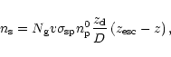 |
(A.4) |
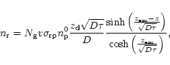 |
(A.5) |
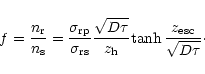 |
(A.6) |
 |
(A.7) |
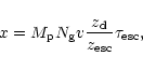 |
(A.9) |
Combining this with Eq. (A.8) we obtain
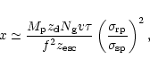 |
(A.10) |
If we include the convection term into the kinetic equation
the analysis becomes more complicated, but the result is almost the same.
If the velocity depends on z as
| V(z)=3 V0 z , | (A.11) |
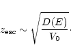 |
(A.14) |
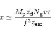 |
(A.15) |
This value estimated from the chemical composition of CRs near Earth is
usually defined as the size of the CR halo. On the other hand the
halo size can be derived from the global ![]() -ray emissivity distribution
in the Galactic plane. The value of
-ray emissivity distribution
in the Galactic plane. The value of
![]() then determines the
size of the CR mixing volume, which is estimated to be at least 10 kpc.
If the diffusion model would describe the CR distribution correctly
and satisfactorily in the Galaxy,
the estimates of
then determines the
size of the CR mixing volume, which is estimated to be at least 10 kpc.
If the diffusion model would describe the CR distribution correctly
and satisfactorily in the Galaxy,
the estimates of
![]() obtained from local and global
data would be similar.
However, the sizes of the CR propagation region differ from each other by
about one order of magnitude, ruling out pure diffusion as the sole CR
transport process.
obtained from local and global
data would be similar.
However, the sizes of the CR propagation region differ from each other by
about one order of magnitude, ruling out pure diffusion as the sole CR
transport process.
Using the transformation formula
 | |||
 |
(B.5) | ||
The Fourier transform
| = |  |
(C.1) |
![$\displaystyle F(\xi=0) = \mp \frac{i \exp(i k \varrho^{\prime})}{2}
\left\{{{\G...
...i\beta}{2}\right) +
\cos\left(\frac{\pi\alpha}{2}\right)\right]}}\right\}
\cdot$](/articles/aa/full/2002/13/aah2935/img468.gif) |
(C.2) |
| = |  |
 | (C.7) | ||
| (C.8) |
 |
(C.9) |
We see from Eq. (C.3) that the contour of integration should be
enclosed in the
semiplane
![]() for
for
![]() ,
i.e. the contour
,
i.e. the contour ![]() in Figs. C.1 and C.2.
In this case the integration over the outer part of the closed contour is
zero and
the function G equals the residues of the sum inside the closed contour only.
For
in Figs. C.1 and C.2.
In this case the integration over the outer part of the closed contour is
zero and
the function G equals the residues of the sum inside the closed contour only.
For
![]() the contour is enclosed in the outer part of the
semiplane
the contour is enclosed in the outer part of the
semiplane
![]() ,
i.e. the contour
,
i.e. the contour ![]() in
Figs. C.1 and C.2.
The locations of the poles in the K-plane are determined from a one-to-one
map of the contours onto the
in
Figs. C.1 and C.2.
The locations of the poles in the K-plane are determined from a one-to-one
map of the contours onto the ![]() - and
- and ![]() -planes and
subsequently Eqs. (C.4) and (C.5) are applied.
-planes and
subsequently Eqs. (C.4) and (C.5) are applied.
The Green's function reads
The contours for
![]() and
and
![]() in the k-plane are
shown for
in the k-plane are
shown for ![]() in Fig. C.1, and for
in Fig. C.1, and for ![]() in Fig. C.2.
in Fig. C.2.
![\begin{figure}
\par\includegraphics[angle=-90,width=7cm,clip]{h2935F8.eps} \end{figure}](/articles/aa/full/2002/13/aah2935/img497.gif) |
Figure C.1:
The contours of integration |
![\begin{figure}
\par\includegraphics[angle=-90,width=7cm,clip]{h2935F9.eps} \end{figure}](/articles/aa/full/2002/13/aah2935/img498.gif) |
Figure C.2:
The contours of integration |
To determine the locations of the poles of the ![]() -functions
-functions
![]() and
and
![]() in the K-plane we should map a unique array of
K values one-to-one onto corresponding arrays of
in the K-plane we should map a unique array of
K values one-to-one onto corresponding arrays of ![]() and
and ![]() values. In this way we
define the contours of
values. In this way we
define the contours of
![]() and
and
![]() in
in
![]() and
and ![]() planes.
planes.
We start with
![]() .
.
![\begin{figure}
\par\includegraphics[angle=-90,width=5.6cm,clip]{h2935F10.eps} \end{figure}](/articles/aa/full/2002/13/aah2935/img503.gif) |
Figure C.3:
The contour of integration |
 |
(C.12) |
Since there is a branch point in the k-plane at
 |
(C.13) |
 |
(C.14) |
 |
(C.15) |
We conclude this section by deriving the transformations between
K-, ![]() - and
- and ![]() -planes, and by deriving the Green's functions
both for strong and weak advection.
From the condition of one-to-one correspondence we obtain
for the poles in the K-plane
-planes, and by deriving the Green's functions
both for strong and weak advection.
From the condition of one-to-one correspondence we obtain
for the poles in the K-plane
| = | (C.16) |
| (C.17) | |||
| = | (C.20) | ||
| = | (C.21) | ||
| Kn | = | (C.22) | |
| = | (C.23) | ||
| = | (C.24) | ||
| = | |||
| (C.25) | |||
| Km | = | (C.26) | |
| = | (C.27) |
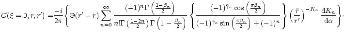 | (C.28) | ||
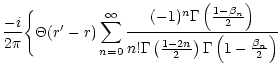 |
|||
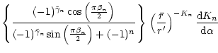 |
|||
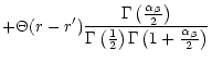 |
|||
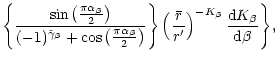 |
(C.29) | ||
| = | 1 | (C.30) | |
| = | (C.31) | ||
| = | (C.32) | ||
| = | (C.33) | ||
| = | (C.34) |
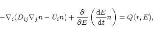
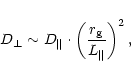
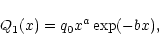
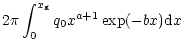
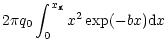
![$\displaystyle 2 \pi q_0 \left[-\exp(-b x) \left({x^2 \over b} + {2 x \over b^2}
+ {2 \over b^3} \right)\right]_{0}^{x_{\rm g}}$](/articles/aa/full/2002/13/aah2935/img72.gif)
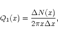


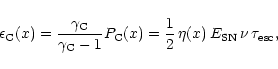
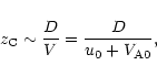
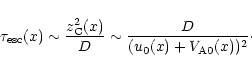
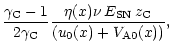
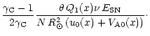
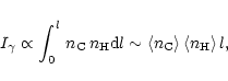
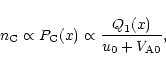
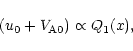
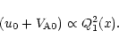
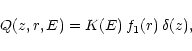
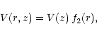
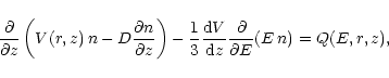
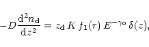
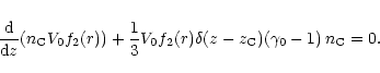
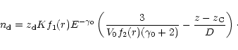
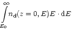
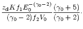
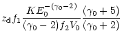
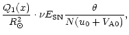
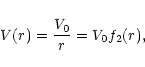
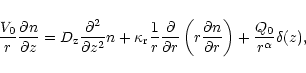


![$\displaystyle \times\exp\left\{-{V_0\over{\sqrt{\kappa_{\rm r} D_{\rm z}}}}\lef...
...left[\sqrt{D_{\rm z} \over\kappa_{\rm r}}{r\over z}\right]\right)\right\} \cdot$](/articles/aa/full/2002/13/aah2935/img229.gif)

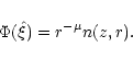
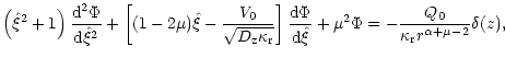
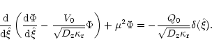
![\begin{displaymath}\left(\hat\xi^2+1\right){{{\rm d}^2\Phi}\over{{\rm d}\hat\xi^...
...r}}}}\right]{{{\rm d}\Phi}\over{{\rm d}\hat\xi}}+\mu^2\Phi=0 .
\end{displaymath}](/articles/aa/full/2002/13/aah2935/img247.gif)


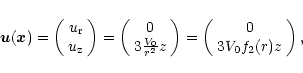


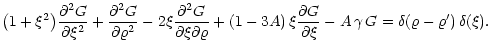
![\begin{displaymath}x (x-1) y^{\prime\prime} + \left[(\alpha+\beta+1) x - \tilde\gamma
\right] y^{\prime} + \alpha \beta y = 0 ,
\end{displaymath}](/articles/aa/full/2002/13/aah2935/img324.gif)
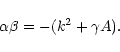


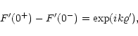
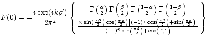
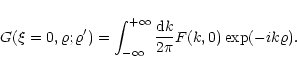
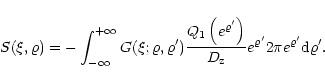
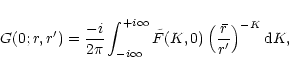
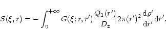

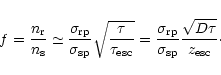

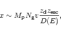

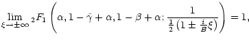
![$\displaystyle {\lim_{\xi \to \pm\infty} \Biggl\{{\rm e}^{i \pi \alpha}
\left[\frac{1}{2}\left(1\pm {i \over B} \xi\right)\right]^{-\alpha}
}$](/articles/aa/full/2002/13/aah2935/img442.gif)
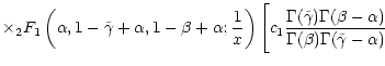
![$\displaystyle + c_2 \, {\rm e}^{- i \pi(\tilde\gamma-1)}
{\Gamma(2-\tilde\gamma...
...(\beta-\alpha) \over \Gamma(\beta -
\tilde\gamma + 1) \Gamma(1-\alpha)} \Biggr]$](/articles/aa/full/2002/13/aah2935/img444.gif)
![$\displaystyle + {\rm e}^{i \pi \beta}
\left[\frac{1}{2}\left(1\pm {i \over B} \xi\right)\right]^{-\beta}$](/articles/aa/full/2002/13/aah2935/img445.gif)
![$\displaystyle + c_2 \, {\rm e}^{- i \pi(\tilde\gamma-1)}
{\Gamma(2-\tilde\gamma...
... \over \Gamma(\alpha -
\tilde\gamma + 1) \Gamma(1-\beta)} \Biggr]\Biggr\} = 0 .$](/articles/aa/full/2002/13/aah2935/img447.gif)
![$\displaystyle \mp \frac{i B \exp(i k \varrho^{\prime})}{2 \sqrt{\pi}}
{(-1)^{\t...
...left(\frac{\pi\beta}{2}\right) +
\cos\left(\frac{\pi\alpha}{2}\right)\right]}
,$](/articles/aa/full/2002/13/aah2935/img463.gif)
![$\displaystyle \times {2^{-(\alpha+\beta)}
\cos\left(\frac{\pi\alpha}{2}\right) ...
...t(\frac{\pi\beta}{2}\right) +
\cos\left(\frac{\pi\alpha}{2}\right)\right]}\cdot$](/articles/aa/full/2002/13/aah2935/img465.gif)
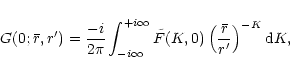

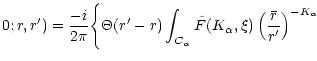
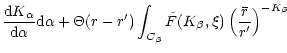

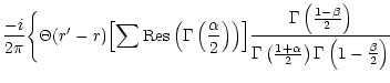
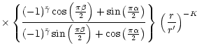
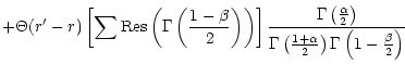
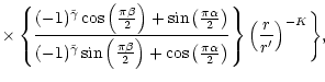
![\begin{figure}
\par\includegraphics[angle=-90,width=5.6cm,clip]{h2935F11.eps} \end{figure}](/articles/aa/full/2002/13/aah2935/img507.gif)
![\begin{figure}
\par\includegraphics[angle=-90,width=5.6cm,clip]{h2935F12.eps} \end{figure}](/articles/aa/full/2002/13/aah2935/img508.gif)