A&A 384, 1119-1123 (2002)
DOI: 10.1051/0004-6361:20011773
Critical Richardson numbers and gravity waves
V. M. Canuto
NASA, Goddard Institute for Space Studies, 2880 Broadway, New York, NY 10025, USA
Dept. of Applied Physics and Mathematics, Columbia University, New York, NY 10027, USA
Received 23 July 2001 / Accepted 7 December 2001
Abstract
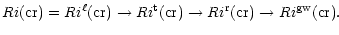
In this paper we present two new results. The first concerns the proper identification of the critical Richardson number Ri(cr) above which there is no longer turbulent mixing. Thus far, all studies have assumed that:
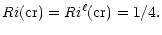 |
|
|
(1) |
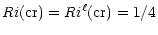
However, since  (cr) determines the upper limit of a laminar regime (superscript
  ), it has little relevance to stars where the problem is not to determine the end point of a laminar regime but the endpoint of turbulence. We show that the latter is characterized by
 ,
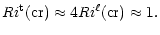
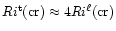
where t stands for turbulence, and has a value four times larger than (1):
,
where t stands for turbulence, and has a value four times larger than (1):
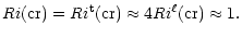 |
|
|
(2) |
We also show that use of (2) instead of (1) changes the conclusions of recent studies.
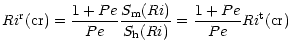
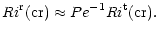
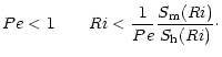
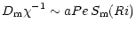
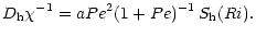
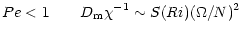
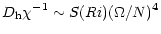
Inclusion of radiative losses (characterized by the Peclet number Pe) which weaken stable stratification and help turbulence, further changes (2) to (r stands for radiative):
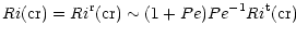 |
|
|
(3) |
which, for Pe<1, allows turbulence to survive far longer than (2). Finally, turbulent convection generates gravity waves that propagate into the radiative region and act as an additional source of energy. This further changes Eq. (3) to (gw stands for gravity waves):
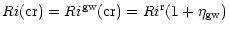 |
|
|
(4) |
where
 .
In conclusion, the successive inclusion of relevant physical processes leads to a chain of increasing values of
.
In conclusion, the successive inclusion of relevant physical processes leads to a chain of increasing values of
 :
:
 |
|
|
(5) |
The second result concerns the dependence of the diffusivity D on  .
We show that the commonly used expression
.
We show that the commonly used expression
 |
|
|
(6) |
is not correct for the regime Pe<1 that characterizes a stably stratified regime. The proper -dependence is:
 |
|
|
(7) |
Key words: Sun: general - Sun: interior - convection - turbulence
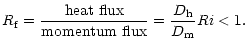
The determination of turbulent diffusivities for a stably stratified, radiative regime in the presence of sources like shear (differential rotation, meridional currents), encompasses several aspects that need to be analyzed. First, since a diffusivity D is of the form:
 |
|
|
(1a) |
where w is an rms velocity and  is a mixing length, one needs to specify two independent variables, w and .
Using Kolmogorov law,
is a mixing length, one needs to specify two independent variables, w and .
Using Kolmogorov law,
 ,
where K is the turbulent kinetic energy and
,
where K is the turbulent kinetic energy and
 is the rate of dissipation of K, Eq. (1a) can be written as:
 |
|
|
(1b) |
which is physically much clearer than (1a). In fact, K has its maximum at the largest scales whereas
(being a dissipation) peaks at the smallest scales. The specification of K and
is therefore equivalent to specifying both large and small scales. Turbulence modeling provides the two dynamic equations satisfied by Kand
(Canuto 1998; Kupka 2001).
The second problem is that a large variety of independent data from laboratory to large eddy simulations (Webster 1964; Istweire & Helland 1989; Schumann & Gerz 1995; Wang et al. 1996; Kosovic & Curry 2000; Strang & Fernando 2001) have shown that stratification has different effects on heat and momentum transport but Eq. (1b) is unable to account for that fact. On the other hand, turbulence models yield the following result:
 |
|
|
(1c) |
where the  (
(
 ,
momentum and heat) are dimensionless structure functions that are different from momentum and heat. The
are functions of:
,
momentum and heat) are dimensionless structure functions that are different from momentum and heat. The
are functions of:
 |
|
|
(1d) |
where Pe is the Peclet number that characterizes radiative losses ( in cm2 s-1 is the radiative diffusivity):
 |
|
|
(1e) |
Ri is the Richardson number:
 |
|
|
(2a) |
characterizing the ratio between sinks (stable stratification N2 and sources (shear instabilities,
 ). Specifically,
  is the mean rate of strain (
 is the mean velocity field)
 |
|
|
(2b) |
and N is the Brunt-Vaisala frequency:
![$\displaystyle %
N^{2} = g\alpha \left[\frac{\partial T}{\partial z} - \left(\fr...
...rtial z}\right)_{\rm ad}\right] = gH_{\rm p}^{-1} (\nabla_{\rm ad} - \nabla)>0.$](/articles/aa/full/2002/12/aa1711/img31.gif) |
|
|
(2c) |
Third, there must exist a critical value Ri(cr) of the Richardson number at which turbulent mixing ceases since stable stratification has become too strong. Operationally, one defines
 (cr) as the value at which the turbulent kinetic energy vanishes:
![$\displaystyle %
K\left[Ri^{\rm t} {\rm (cr)}\right] = 0$](/articles/aa/full/2002/12/aa1711/img33.gif) |
|
|
(2d) |
and Eq. (1c) implies that the diffusivities also vanish at
(cr). Given the above procedure and a turbulence model that provides the functions:
 |
|
|
(2e) |
the value of
(cr) is given by solving (2d) and need not be imposed. When no turbulence model is available and the diffusivities are constructed using heuristic arguments, the lack of a dynamic equation for K deprives such models of Eq. (2d) and
(cr) must be guessed, a procedure that has been used thus far, as we discuss next.
Lacking a turbulence model, in all astrophysical literature thus far (Zahn 1974; Pinsonneault et al. 1989; Meader 1995; Meader & Meynet 1996; Garcia-Lopez & Spruit 1991; Talon & Zahn 1997; Schatzman et al. 2000), it has been customary to identify:
 |
|
|
(3a) |
where
 |
|
|
(3b) |
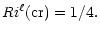
Equation (3b) was derived by Miles (1961) and Howard (1961) using linear stability analysis and represents the value at which a laminar flow (thus the superscript )
becomes unstable. In what follows, several arguments are presented to show that, given the specific task of identifying when, in a stably stratified region of a star, turbulent mixing ceases to exist, Eqs. (3a), (3b) are not the correct answer.
First, Eq. (3b) is the result of a "road from laminarity'', an approach that can only tell us when a linear regime breaks down and non-linearities becom important. When that occurs, one first enters a weakly non-linear regime and then finally in a turbulent regime where the non-linearities dominate. We refer the reader to an illustrative depiction of these successive processes (Woods 1969) which highlights the different physical regimes of laminar, weakly non-linear and strongly non-linear regimes. Given a stable laminar sheet of thickness h, Kelvin-Helmholtz instabilities gradually erode and entrain fluid parcels above and below h. The process leads to an incrase of h which ceases when the thickness has become about four times the original value h. Woods (1969) concluded that "since the final thickness is nearly four times the original value, the final Richardson number is also four times the value prior to the instability''. The turbulent Richardson number
is thus computed to be:
 |
|
|
(3c) |
Equation (3c) has also been derived using other arguments. Once the regime described by (3b) has been crossed, non-linearities become important and one must carry out a stability analysis including them. Abarbanel et al. (1984) proved that in such a case the sufficient and necessary condition for instability is:
 |
|
|
(3d) |
which agrees with the heuristic argument leading to (3c).
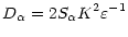
A more physical argument relies on energy considerations. A turbulent state can be maintained only as long as the sources outweigh the sinks. Using the equation for the turbulent kinetic energy (Canuto 1998), this criterion becomes:
 |
|
|
(4a) |
where  is the "flux Richardson number'' defined as (see Eqs. (9b)-(9d)):
 |
|
|
(4b) |
Thus, Eq. (4a) becomes:
 |
|
|
(4c) |
Martin (1985) showed that the computed oceanic upper mixed layer (which is strongly stable and stirred by shear) could match observations only if (3d) was satisfied. Large eddy simulation of a stable planetary boundary layer by Kosovic & Curry (2000) also conclude that mixing exists up to
 .
A number of other cases leading to (3d) are discussed in Strang & Fernando (2001).
.
A number of other cases leading to (3d) are discussed in Strang & Fernando (2001).
From the turbulence modeling viewpoint, turbulence models (Canuto 1998) provide the dependence of the turbulent kinetic energy K on Ri. Since the stronger the degree of stability, the harder it is for turbulence to survive, K is a decreasing function of Ri and at some
,
Eq. (2d) is satisfied and the value of
so identified. The solution of Eq. (2d) was obtained in (Canuto 1998, Fig. 6a) and the result agrees with (3c):
 |
|
|
(4d) |
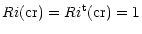
In conclusion,
 and
represent two different physical situations. In laboratory experiments one follows the development of an instability and witnesses the transition from a laminar to a weakly non-linear state, a bottom-up approach that confirms
as the transition value. However, in stars one cannot follow such a development and one must therefore adopt a conceptually different approach, a top-down approach. One is presented with a situation in which there is turbulent mixing and the relevant question then changes to: what is maximum value of Ri for which such mixing can be sustained? Since turbulent mixing is due to strong non-linearities, the answer is
and
represent two different physical situations. In laboratory experiments one follows the development of an instability and witnesses the transition from a laminar to a weakly non-linear state, a bottom-up approach that confirms
as the transition value. However, in stars one cannot follow such a development and one must therefore adopt a conceptually different approach, a top-down approach. One is presented with a situation in which there is turbulent mixing and the relevant question then changes to: what is maximum value of Ri for which such mixing can be sustained? Since turbulent mixing is due to strong non-linearities, the answer is
 .
Use of
to characterize the boundary between turbulent mixing and no mixing is incorrect since
refers to a physical situation quite different from the one most astrophysical studies intend to describe.
.
Use of
to characterize the boundary between turbulent mixing and no mixing is incorrect since
refers to a physical situation quite different from the one most astrophysical studies intend to describe.
In conclusion, one should forgo the bottom-up approach leading to
and adopt the top-down approach that leads to
.
At first sight, the change from 1/4 to 1 may seem marginal but it is not so, as we now discuss. Garcia-Lopez & Spruit (1991) showed that for gravity waves to be a source of mixing compatible with the data on Li7 depletion, their result had to be boosted by an arbitrary factor of
 which meant that gravity waves mixing is inefficient. However, had the authors used
instead of
,
the boosting factor would have been only
which meant that gravity waves mixing is inefficient. However, had the authors used
instead of
,
the boosting factor would have been only
 ,
which is well within the uncertainties of the problem. Their conclusion would have been that gravity waves are an efficient source of mixing. More recently, Schatzman et al. (2000, SZM) studied whether mixing may be due to shear instabilities. They concluded that for that to occur (their Eq. (8)):
,
which is well within the uncertainties of the problem. Their conclusion would have been that gravity waves are an efficient source of mixing. More recently, Schatzman et al. (2000, SZM) studied whether mixing may be due to shear instabilities. They concluded that for that to occur (their Eq. (8)):
 |
|
|
(5a) |
where  and
are the molecular viscosity and radiative conductivity. SZM used:
and
are the molecular viscosity and radiative conductivity. SZM used:
 |
|
|
(5b) |
and showed (their Fig. 2) that  almost never satisfies (5a). Had SZM used:
 |
|
|
(5c) |
the first relation in (5a) would have been satisfied and SZM would have concluded that shear instabilities do set in. Whether shear instabilities are sufficiently strong to explain the diffusiviy required to explain the depletion of Li7 is a different matter since the quantification of how much mixing is produced by an instability requires a model much more complex than linear analysis, that is, a turbulence model.
As we stressed earlier, the solution of the Reynolds stress equations provided by a turbulence models (Canuto 1998) yields not only the form (1c) but the structure functions
as well. Equation (4c) can therefore be written as (r stands for radiative losses):
 |
|
|
(6a) |
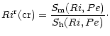 |
|
|
(6b) |
The Pe-dependence of the functions
is such that:
 |
|
|
(7a) |
Both
 are independent of Pe. In the opposite case:
 |
|
|
(7b) |
 is still Pe-independent while
 depends linearly on Pe. Combining (7a,b) into a single expression and substituting into (6b), we obtain:
 |
|
|
(8a) |
which, in the limit of small Pe, yields:
 |
|
|
(8b) |
Thus,
 can be much larger than
.
Using (8a), we rewrite (6a) as:
can be much larger than
.
Using (8a), we rewrite (6a) as:
 |
|
|
(8c) |
In principle, once we add to the previous formalism the dynamic equations for K and
,
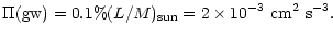
the model is complete. The results can be found in Canuto (1998). However, such an approach, while complete from the point of view of turbulence modeling, does not take into account the presence of gravity waves which are generated in the convective zone and propagate into the radiative zone with a flux  (gw). Such waves act a source of turbulence (in addition to that of shear e.g., differential rotation and meridional currents). In the solar case, Kumar et al. (1999) have computed the flux of gravity waves to be:
 |
|
|
(9a) |
The question then arises: how can one include
into a turbulence model? Here, we suggest a first approach. Consider the stationary limit of the time dependent equation for the turbulent kinetic energy (Canuto 1998, Eq. (25a)):
 |
|
|
(9b) |
where:
 |
|
|
(9c) |
The first term represents the source due to shear (e.g., differential rotation, meridional currents), the second term is the sink due to stable stratification and the third term is the contribution of gravity waves. Using the following forms for the Reynolds stresses  and the heat flux
 (Canuto 1998, Eqs. (39a) and (43a)):
![$\displaystyle %
\tau_{ij}= - 2D_{\rm m} \Sigma_{ij},\quad \overline{w\theta} = ...
...}{\partial z} - \left(\frac{\partial T}{\partial z}\right)_{\rm ad}\right]\cdot$](/articles/aa/full/2002/12/aa1711/img71.gif) |
|
|
(9d) |
Equations (9b), (9c) become:
 |
|
|
(10a) |
which can be written as:
 |
|
|
(10b) |
where the gravity wave-dependent flux Richardson number is defined as:
 |
|
|
(10c) |
which replaces (4b). Using (6b), we obtain:
 |
|
|
(10d) |
where:
 |
|
|
(10e) |
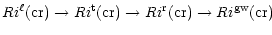
Thus, in the presence of gravity waves,
Rigw(cr) is larger than
Rir(cr).
The expression for the scalar turbulent diffusivity D employed thus far in the literature does not differentiale between momentum and heat. Its specific form has been taken to be:
 |
|
|
(11a) |
where and  stands for .
Equation (11a) has been widely used (Baglin et al. 1985; Maeder 1995; Maeder & Meynet 1996; Talon & Zahn 1997; Charbonnel & Talon 1999).
stands for .
Equation (11a) has been widely used (Baglin et al. 1985; Maeder 1995; Maeder & Meynet 1996; Talon & Zahn 1997; Charbonnel & Talon 1999).
Let us repeat the standard derivation of (11a) keeping the
structure functions. Starting with (1c) and using (1e), one has
 :
:
 |
|
|
(11b) |
For momentum and heat diffusivities, we have:
Because of (7a), (7b), we can further write for any Pe:
 |
|
|
(11e) |
 |
|
|
(11f) |
The different Pe-dependence of  and
and  is a result that was first derived by Howells (1960) using heuristic arguments and later proven rigorously with RNG (Renormalization group; Canuto & Dubovikov 1996, Eqs. (C16-18)). Next, we employ (8c) to eliminate Pe and obtain:
 |
|
|
(12a) |
 |
|
|
(12b) |
where the function S(Ri)
 |
|
|
(12c) |
is plotted in Fig. 1. When compared with (11a), the new expressions (12) exhibit several new features:
- 1)
- heat and momentum diffusivity are different,
- 2)
- only the momentum diffusivity scales like
 ,
,
- 3)
- heat diffusivity scales like
 ,
,
- 4)
- the absence of the
functions in phenomenological models means that they lack the function S(Ri) which ensures that the diffusivities vanish at some point (Fig. 1),
- 5)
- the value at which
 vanish is represented by the variable S(Ri), see Fig. 1. The point at which the diffusivities vanish corresponds to the value of Ri at which the turbulent kinetic energy vanishes.
In summary, the above derivation shows the major differences brought about by the structure fonctions
vis à vis the standard model where they are absent.
![\begin{figure}
\par\includegraphics[width=6.3cm,clip]{fig1.eps}\end{figure}](/articles/aa/full/2002/12/aa1711/Timg96.gif) |
Figure 1:
The function S(Ri) defined in Eq. (12c) is plotted vs. the Richardson number Ri. As one can observe, turbulence exists way past the Ri= 1/4 value. It dies only at  . . |
| Open with DEXTER |
Several arguments have been presented to show that in a stably stratified fluid, shear dominated turbulence persists above the laminar value
 .
Regrettably, the lack of a turbulence model has prompted the use of the laminar value
in spite of the fact that it does not represent the physical situation encountered in stellar interiors.
.
Regrettably, the lack of a turbulence model has prompted the use of the laminar value
in spite of the fact that it does not represent the physical situation encountered in stellar interiors.
The bottom-up approach starting from linear stability and leading to
must be substituted with a top-down approach that gives the range of values of Ri for which turbulent mixing operates. The new
is defined as the value at which turbulence ceases to exist since the turbulent kinetic energy vanishes. Several independent arguments are presented to show that:
 |
|
|
(13a) |
a value that would have changed the conclusions of Schatzman et al. (2000) and considerably strengthen the conclusions of Garcia-Lopez & Spruit (1991) concerning gravity waves as a source of mixing.
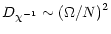
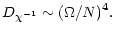
Radiative losses further increase the critical
to
which for Pe <1 is
 times larger than (13a). Gravity waves act as a source of mixing leading to a further boost in the value of
.
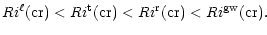
Through the successive inclusion of physical processes we have shown the sequence:
times larger than (13a). Gravity waves act as a source of mixing leading to a further boost in the value of
.
Through the successive inclusion of physical processes we have shown the sequence:
 |
|
|
(13b) |
with
 |
|
|
(13c) |
In conclusion, the traditional
 must be replaced by
Ri gw (cr).
must be replaced by
Ri gw (cr).
In many ways, the new formalism resolves the dichotomy that has existed thus far between shear-dominated and gravity wave-dominated scenarios. Both processes have been integrated into a single formalism. Numerical results leading to numerical values of the scalar diffusivity D are presented in an upcoming paper (Canuto & Minotti 2001).
Acknowledgements
The author would like to thank an anonymous referee for inquisitive questions that helped improve the original manuscript.
- Abarbanel, H. D., Holm, D. D., Marsden, J. E., & Ratiu, T. 1984, Phys. Rev. Lett., 52, 2352
In the text
NASA ADS
- Baglin, A., Morel, P. J., & Schatzman, E. 1985, A&A, 149, 309
In the text
NASA ADS
- Canuto, V. M. 1998, ApJ, 508, 767
In the text
NASA ADS
- Canuto, V. M., & Dubovikov, M. S. 1996, Phys. Fluids, 8, 571
In the text
NASA ADS
- Canuto, V. M., & Dubovikov, M. S. 1998, ApJ, 493, 834
NASA ADS
- Canuto, V. M., & Minotti, F. 2001, MNRAS, submitted
In the text
- Charbonnel, C., & Talon, S. 1999, A&A, 351, 635
In the text
NASA ADS
- Garcia-Lopez, R. J., & Spruit, H. 1991, ApJ, 377, 368
In the text
- Gerz, T., Schumann, U., & Elgobashi, S. E. 1989, J. Fluid Mech., 200, 563
NASA ADS
- Howard, L. N. 1961, J. Fluid Mech., 10, 509
In the text
NASA ADS
- Howells, I. D. 1960, JFM, 9, 104
In the text
- Itsweire, E. C., & Helland, K. N. 1989, J. Fluid Mech., 207, 419
- Kosovic, B., & Curry, J. A. 2000, J. Atmos. Sci., 57, 1052
In the text
- Kumar, O., Talon, O., & Zahn, J. P. 1999, ApJ, 520, 859
In the text
NASA ADS
- Kupka, F. 2001, ApJ, submitted
In the text
- Maeder, A. 1995, A&A, 299, 84
In the text
NASA ADS
- Maeder, A., & Meynet, G. 1996, A&A, 313, 140
In the text
NASA ADS
- Martin, P. J. 1985, J. Geophys. Res., 90, 903
In the text
NASA ADS
- Miles, J. W. 1961, J. Fluid Mech., 10, 496
In the text
- Pinsonneault, M. H., Kawaler, S. D., Sofia, S., & Demarque, P. 1989, ApJ, 338, 424
In the text
NASA ADS
- Schatzman, E., Zahn, J. P., & Morel, P. 2000, A&A, 364, 876
In the text
NASA ADS
- Schumann, U., & Gerz, T. 1995, J. Appl. Met., 34, 33
In the text
- Strang, E. J., & Fernando, H. J. S. 2001, J. Phys. Oceanogr., 31, 2026
In the text
- Talon, S., & Zahn, J. P. 1997, A&A, 317, 749
In the text
NASA ADS
- Wang, D., Large, W. G., & McWilliams, J. C. 1996, J. Geophys. Res., 101, 3649
In the text
NASA ADS
- Webster, C. A. G. 1969, J. Fluid Mech., 19, 221
- Woods, J. D. 1969, Radio Science, 4, 1289
In the text
- Zahn, J. P. 1974, in Stellar Instability and Evolution, ed. P. Ledoux, A. Noels, & W. Rodgers (Dordrecht, Reidell), IAU Symp., 59, 185
In the text
Copyright ESO 2002
![\begin{figure}
\par\includegraphics[width=6.3cm,clip]{fig1.eps}\end{figure}](/articles/aa/full/2002/12/aa1711/img96.gif)