A&A 384, 414-432 (2002)
DOI: 10.1051/0004-6361:20020044
J. Pétri 1 - J. Heyvaerts 1 - S. Bonazzola 2
1 - Observatoire de Strasbourg,
11 rue de l'Université,
67000 Strasbourg, France
2 -
DARC, Observatoire de Meudon,
Place Jules Janssen,
92195 Meudon, France
Received 21 August 2001 / Accepted 14 December 2001
Abstract
In this paper we present self-consistent models of the magnetosphere
of inactive, charged, aligned rotator pulsars. We have devised an
efficient semi-analytical and numerical algorithm to construct such
models. The only free parameter is the total charge of the system.
These charge-separated "electrospheres" consist of an equatorial
belt carrying charge of one sign, partially in differential
rotation, and of two oppositely charged domes located over the poles
which corotate with the neutron star. The dependence of the shape
of these plasma-filled regions surrounding the star on the total
charge of the system and of their differential rotation is
investigated. It is shown that our solutions are stable to vacuum
breakdown by electron-positron pair production in most of the
light-cylinder volume, except perhaps in the case of millisecond
pulsars. The small regions where vacuum breakdown occurs are shown
to behave merely as an effective extension of the star's volume. We
have also found that no permanent null-charged wind emanating from
the polar caps can exist in a stationary state. Indeed, for a given
total charge of the system determined by the net outgoing charged
flux, the potential configuration becomes unfavorable to particles
escaping to infinity. Finally, we have shown that the geometric and
kinematic structure of the electrosphere is uniquely determined by
the total charge of the system.
Key words: stars: pulsars: general - plasmas - MHD - methods: numerical
The magnetosphere of an isolated solid star or planet rotating in a vacuum seemingly has a very simple structure, being just the external vacuum region of a spinning spherical conducting magnet. However, in the regime appropriate to fast rotating magnetized neutron stars, it is a lot more complex. In a similar laboratory setup, electric charge would be distributed in the conducting body, in particular at its surface as surface-charges that would be retained in the body by a large enough extraction potential. It has however been recognized that such surface charges can be extracted even from the very magnetized crust of neutron stars by the intense electric field which appears at its surface (Goldreich & Julian 1969). We assume this to be equally true for electrons and ions, although the case is less clear for iron nuclei than it is for electrons (Ruderman & Sutherland 1975). Then the external region does not remain void. The determination of the structure of fields and charged flows outside of the star still remains a partially unsolved problem.
This paper, and the following in this series, aim at defining the electric structure of isolated neutron star magnetospheres in different physical regimes. We consider here the aligned rotator model of a pulsar, in which the magnetic field of the star is dipolar. Following Goldreich & Julian (1969), the stationary state reached by this system is usually viewed as consisting of a closed magnetosphere and open magnetic field structures rooted at its polar caps. Both regions are supposedly filled with electron-positron plasma, except perhaps at very small gaps. An outwards charged relativistic plasma wind is assumed to be present on field lines rooted at the polar caps that reach the light cylinder and extend beyond it. The physics of this relativistic wind has been extensively studied (Michel 1973, 1974; Goldreich & Julian 1970; Beskin et al. 1993) and is still the subject of active research concerning the geometry of the flow (Li et al. 1992; Bogovalov 2001) and the self-consistent determination of the total current in the system (Contopoulos et al. 1999). Unless the star is heavily charged, the sign of the extracted charges is, in the case of a dipolar field, uniform and the same over both northern and southern polar caps. The system would then globally lose charge unless the current somehow closes back on the star. Ways of achieving this have been suggested (Mestel 1984; Hofmann et al. 1996; Beskin et al. 1993) which all rely on relativistic processes such as radiation reaction or the breakdown of the electric drift approximation. Otherwise, there would be a steady charging up of the star until net charge loss is quenched by the growing unipolar electric field and the star's environment finds a state of electrostatic equilibrium.
This latter view of neutron star's environment has also been studied by a number of authors but has altogether received less attention than plasma-filled magnetospheres and pulsar wind models. This is due in part to the fact that an aligned rotator pulsar in a state of electrostatic equilibrium is inactive. In wind models, the space around the neutron star is supposedly entirely filled with leptonic plasma that must be self consistently produced by a pair avalanche process. This raises the question of what happens when pair creation activity ceases or when it is not possible, and also of what aligned rotators would look like if pair creation did not exist at all.
Here we study the structure of the environment of rotating neutron stars that have reached a state in which axisymmetric rotating charged plasma has found an equilibrium between the electromotive and electric fields, partly self-generated, in which it is sitting. This we describe for brevity as an electrostatic equilibrium. We refer to the associated solution as an electrosphere. We shall rely on the electrostatic approximation, neglecting self-created magnetic fields generated by the rotating charged plasma. This is correct as long as the electrosphere remains confined to well within the light cylinder.
The limits of "activity" in the parameter space of aligned rotating neutron stars is set by the stability of these inactive structures both to vacuum sparking, which we discuss in this paper, and to global electromagnetic perturbations which we shall discuss in a forthcoming paper. The construction of stationary models is a prerequisite to this study.
In Goldreich and Julian's picture (1969), the closed magnetosphere is in electrostatic equilibrium and all its volume is filled with charged plasma. This view has been challenged, and the possibility of extended vacuum gaps has been discussed by many authors (Holloway 1973; Holloway & Pryce 1981; Ruderman & Sutherland 1975; Cheng et al. 1976). It has even been shown that a closed magnetosphere contained within the light cylinder and totally plasma filled is unstable to the opening of wide gaps between the positively and negatively charged regions (Thacker et al. 1998).
The effect of a net total charge of the neutron star has been considered by Jackson (1976) who has shown that domes consisting of electrically trapped charged particles are then likely to form above the star's polar regions. Jackson did not obtain a complete self consistent solution, though. Pilipp (1974) made the important point that no consistent solution exists in which the electrosphere would only consist of plasma surrounding the star and corotating with it, whatever the shape of the interface of the plasma filled region with the surrounding vacuum. Pilipp's theorem does not exclude the possibility that the electrosphere consists of a corotating part, connected to the star itself, and a region separated from it by a certain potential drop along field lines. This latter region would in general be differentially rotating.
The first successful attempt at finding a completely self consistent solution for the structure of an electrosphere was made by Krause-Polstorff & Michel (1985a, 1985b), who numerically conducted an experiment by which a number of annular shaped charges are transfered to the magnetosphere and naturally find an equilibrium position. Due to the use of a limited number of charges their results were somewhat noisy. In this paper we elaborate on their approach in the same spirit by building up the electrosphere numerically by a recurrence process which however does not consist in transferring a limited number of "point" charges. Other authors (Shibata 1989a,1989b) have conducted similar numerical constructions, but did not calculate the differentially rotating part of the electrosphere, a most important aspect with which we deal here.
Our study considers an aligned rotator with a dipolar magnetic
field. We assume that the external fields and flows share the axisymmetry of
the driving setup. For their description we either use cylindrical
coordinates (
![]() )
or spherical coordinates (
)
or spherical coordinates (
![]() )
built on the rotation axis, the angle
)
built on the rotation axis, the angle ![]() being the
colatitude. Unit vectors of the corresponding
local frames are denoted by
being the
colatitude. Unit vectors of the corresponding
local frames are denoted by ![]() with a subscript, such as
with a subscript, such as
![]() say. Physical quantities are expressed in the MKSA system of
units,
say. Physical quantities are expressed in the MKSA system of
units,
![]() being the dielectric permittivity of vacuum and
being the dielectric permittivity of vacuum and
![]() its magnetic permeability.
its magnetic permeability.
An electrosphere is a charge distribution in which, wherever there is plasma, the electric field component aligned to the magnetic field vanishes, just as it does in the supposedly perfectly conducting star itself. The electrospheric plasma is regarded as cold (models of hot charge-separated electrospheres have been calculated by Neukirch 1993). This plasma can be distributed in volumes separated by vacuum regions, which we refer to as vacuum gaps, or gaps for short. The vacuum/cold plasma interface is sharp. At equilibrium this interface should be force free in the sense that there should be no electric force acting along the direction of the magnetic field at it. In the gaps the electric potential is a solution of Laplace's equation and the electric field may have a component along the magnetic field. Another requirement is that the solution be accessible, in the sense that there exist some physically possible way of building it up by transferring the charges from the star to where they should eventually be found, starting from, say, an initial state where there is vacuum outside of the star.
The following assumptions are used throughout the paper:
Let us now describe our iterative scheme to converge to a solution and introduce the physical quantities which characterize the structure of an electrosphere. We assume the initial situation to be that which exists when electric charges have not escaped out of the star's crust. The corresponding external and internal electric potentials are easily obtained. Our algorithm then works along the following steps:
We begin by considering a conducting sphere, source of a dipolar
magnetic field, rotating at a rate
![]() surrounded by vacuum.
The dipolar magnetic field at a point of spherical coordinates (R,
surrounded by vacuum.
The dipolar magnetic field at a point of spherical coordinates (R,
![]() )
is expressed as:
)
is expressed as:
 |
(6) |
To proceed with the iteration, we must calculate at each step the most
significant quantity which is the electric potential ![]() outside of
the star. We split this quantity into two parts, the first one being
the vacuum electric potential created by the charges present inside
the neutron star and at its surface, noted
outside of
the star. We split this quantity into two parts, the first one being
the vacuum electric potential created by the charges present inside
the neutron star and at its surface, noted
![]() ,
and the second
one being the electrospheric potential,
,
and the second
one being the electrospheric potential,
![]() ,
created by the
charges present in the external region. Inside the star the total
potential is the corotation potential
,
created by the
charges present in the external region. Inside the star the total
potential is the corotation potential
 |
(13) |
 |
(14) |
| k2 | = |  |
(15) |
| l2 | = |  |
(16) |
The stellar surface charge density
![]() is again obtained from
the discontinuity of the component of the electric field normal to the
star's surface,
is again obtained from
the discontinuity of the component of the electric field normal to the
star's surface,
![]() ,
which is easily
expressed in terms of
,
which is easily
expressed in terms of
![]() by:
by:
 |
(18) |
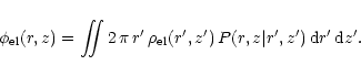
In the plasma-filled region the relation (1) implies
that magnetic field lines are equipotentials so that the electric
potential ![]() in these regions is a function
in these regions is a function ![]() of the flux
variable a. The associated electric field is
of the flux
variable a. The associated electric field is
 |
(19) |
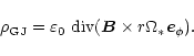
In a closed magnetosphere corotating with the star at the angular
velocity ![]() the charge density is the so-called
Goldreich-Julian value
the charge density is the so-called
Goldreich-Julian value
![]() ,
the value of which results from
assuming local electrostatic equilibrium with the electromotive field,
so that
,
the value of which results from
assuming local electrostatic equilibrium with the electromotive field,
so that
 |
(24) |
At each step of the iterative construction of the solution we know how
much charge,
![]() da and
da and
![]() da resp., is contained in the
equatorial belt region (hereafter referred to as "the disk", subscript
D) and in each polar dome (subscript P) in the flux tube between
the magnetic surfaces a and a +da (see
Fig. 1).
da resp., is contained in the
equatorial belt region (hereafter referred to as "the disk", subscript
D) and in each polar dome (subscript P) in the flux tube between
the magnetic surfaces a and a +da (see
Fig. 1).
![\begin{figure}
\par\includegraphics[width=8.8cm,clip]{MS1831f1.pstex} \end{figure}](/articles/aa/full/2002/11/aa1831/img94.gif) |
Figure 1:
Schematic representation of the geometrical shape of the
electrosphere, illustrating the definition of the parameters
|
| Open with DEXTER | |
Nothing has been said about the mechanism of extraction of particles from the pulsar crust. This is because this physics is irrelevant to the mathematical iteration process by which our solutions are constructed. It is only demanded that charge extraction and transfer be indeed physically possible. The question of feasibility of charged particle emission from the surface of a neutron star is still unsolved due to the unknown value of the work function. Attempts have been made to estimate this function (Flowers et al. 1977) but yield different results (Müller 1984; Neuhauser 1987). According to Jones (1986), the cohesive energy of the atomic lattice is roughly several hundred eV. This energy range is reached for surface temperatures T=106-107 K, which are believed to be the temperatures of the radio-pulsar crust after cooling. Therefore we conclude that the surface temperature of the star is large enough to allow ionic (even iron nuclei) and electronic thermo-emission from the entire stellar crust. If however the extraction of the heavy ions were to be impossible, only the two electronically charged domes would subsist for an aligned rotator. For an anti-aligned rotator, only the equatorial disc would remain. Its structure would not be drastically altered by the absence of the dome. In what follows, we adopt Jones work function energy which implies easy charge extraction whatever their nature.
How our algorithm progressively transfers charges from the surface of
the rotating neutron star to its electrosphere is described by a
transfer function,
![]() ,
which we made to depend on the
colatitude of charge extraction
,
which we made to depend on the
colatitude of charge extraction ![]() ,
where the surface charge
density currently is
,
where the surface charge
density currently is
![]() ,
and on the number of the
iteration step
,
and on the number of the
iteration step ![]() .
It is defined as being the ratio of the
surface charge, d
.
It is defined as being the ratio of the
surface charge, d
![]() ,
extracted from the pulsar's surface
between colatitudes
,
extracted from the pulsar's surface
between colatitudes ![]() and
and
![]() at iteration step
at iteration step
![]() to the surface charge d
to the surface charge d
![]() d
d![]() present at this step between
these colatitudes. So,
present at this step between
these colatitudes. So,
In order to keep all quantities close to unity in our simulations and
to avoid floating-point overflow, our calculations are performed in
normalized units that refer to the radius ![]() ,
the polar magnetic
field strength
,
the polar magnetic
field strength ![]() and to the angular velocity
and to the angular velocity
![]() .
Since we take no relativistic effect into account, the speed of light
and the light cylinder radius play no explicit role and these three
quantities act only as scaling factors. They do not alter anything but
scales in the physical results when varied. All units derive
naturally from them. In particular, the reference value for electric
charge is
.
Since we take no relativistic effect into account, the speed of light
and the light cylinder radius play no explicit role and these three
quantities act only as scaling factors. They do not alter anything but
scales in the physical results when varied. All units derive
naturally from them. In particular, the reference value for electric
charge is
![]() .
The central
point charge
.
The central
point charge ![]() expressed in this unit is
expressed in this unit is ![]() .
.
The system has been investigated for values of the total charge which
are a multiple of this central point charge of the star. The only
parameter which really affects the structure of the equilibrium
electrosphere is the total charge of the system
![]() .
.
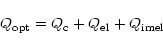
We computed several models with different values of this parameter but we will only discuss here a few among the most representative ones.
Figure 2 shows the main characteristics of a
static electrosphere with
![]() .
.
![\begin{figure}
\par\includegraphics[width=12.9cm,clip]{MS1831f2.eps} \end{figure}](/articles/aa/full/2002/11/aa1831/img112.gif) |
Figure 2:
Main characteristics of the electrosphere for the model with a
total charge
|
| Open with DEXTER | |
A second example, with
![]() ,
is represented in
Fig. 3.
,
is represented in
Fig. 3.
![\begin{figure}
\par\includegraphics[width=12.9cm,clip]{MS1831f3.eps} \end{figure}](/articles/aa/full/2002/11/aa1831/img116.gif) |
Figure 3:
Main characteristics of the electrosphere for the model with total
charge
|
| Open with DEXTER | |
The differences just noted illustrate a general trend. Indeed,
beginning with a model with a low total charge, an increase in the
value of
![]() shrinks the polar regions while it expands the
equatorial disk, also causing an increase of the differential rotation
rate. This is explained by the fact that filling up the belt increases
the radially outward component of the electric field and causes a
faster particle drift motion. As a consequence the rotation rate
increases.
shrinks the polar regions while it expands the
equatorial disk, also causing an increase of the differential rotation
rate. This is explained by the fact that filling up the belt increases
the radially outward component of the electric field and causes a
faster particle drift motion. As a consequence the rotation rate
increases.
Another set of models has been computed, removing the dome. This means that negative surface charge has not been transfered from the star to the electrosphere, and therefore such models retain some surface charge at some places on the star's surface. We found that the structure of the equatorial region had not been drastically perturbed, though. We conclude that the domes have only a minor effect on the structure of the differentially rotating disk (domes only make it possible to bring more ions in the belt).
Replacing the dipolar magnetization by an uniform one in the pulsar makes it impossible to achieve convergence to any equilibrium state. A large amount of positive charge remains present on the surface due to a sharp discontinuity in the electric field component normal to the interface star-electrosphere, the complete disappearance of which appears to be impossible. This is due to the fact that the electric currents which generate the magnetic field are in this case flowing on the surface of the neutron star and not at a central singularity as in the case of a dipolar field. The electric charge density associated with these currents (see Eq. (23)) consequently has in this case a surfacic type of singularity on the star's surface which is inherent to this particular magnetic structure and cannot be removed.
It is important to stress that our solutions are independent of how
charges are transfered from the star to the electrosphere. Indeed,
different choices of transfer function, taking for example
![]() in Eq. (28) to depend
linearly or quadratically on the surface charge density with different
multiplicative factors have been tested to cause no change in the
results shown above. So the solution to which our algorithm converges
is unique. Indeed, as shown in Appendix B, the solution to
the electrosphere structure is unique for a given value of
in Eq. (28) to depend
linearly or quadratically on the surface charge density with different
multiplicative factors have been tested to cause no change in the
results shown above. So the solution to which our algorithm converges
is unique. Indeed, as shown in Appendix B, the solution to
the electrosphere structure is unique for a given value of
![]() .
.
We emphasize the fact that in all these models the gaps are stable in the sense that if somehow a particle were to be found or created in the gap it would be attracted to the region of the electrosphere with the same charge sign as its own and repelled from the region of opposite sign. This is why gaps actually exist (Holloway 1973). So no electric current is to flow from one to the other charge-separated region, unless the system were to suffer large amplitude perturbations.
We summarize below the essential features of the results thus far obtained:
![\begin{figure}
\par\includegraphics[width=13.3cm,clip]{MS1831f4.eps} \end{figure}](/articles/aa/full/2002/11/aa1831/img125.gif) |
Figure 4:
Main characteristics of the electrosphere for the model with null
total charge
|
| Open with DEXTER | |
The neutron star gravitational radius,
![]() ,
is, for
typical neutron star parameters, of order
,
is, for
typical neutron star parameters, of order
![]() which
is not much less than the star's radius. The space-time is thus
strongly curved in the neighborhood of the neutron star surface. This
will alter the structure of the electromagnetic field as compared to
our classical calculation. It has been shown that for a slowly
rotating black hole metric (described by the Kerr metric expanded to
first order in the stellar angular momentum J*, which is a good
approximation if J*/M* is small) the correction in the magnetic
field as compared to the Minkowski flat space-time case is small. The
still dipolar field is increased in magnitude by roughly 10%. To
first order in J*, only the electric field is enhanced by the
inertial frame dragging effect (Rezzolla et al. 2001).
which
is not much less than the star's radius. The space-time is thus
strongly curved in the neighborhood of the neutron star surface. This
will alter the structure of the electromagnetic field as compared to
our classical calculation. It has been shown that for a slowly
rotating black hole metric (described by the Kerr metric expanded to
first order in the stellar angular momentum J*, which is a good
approximation if J*/M* is small) the correction in the magnetic
field as compared to the Minkowski flat space-time case is small. The
still dipolar field is increased in magnitude by roughly 10%. To
first order in J*, only the electric field is enhanced by the
inertial frame dragging effect (Rezzolla et al. 2001).
Adapting our algorithm to curved space-time would imply replacing the
dipolar magnetic field by its general relativistic expression. The
situation for an aligned rotator would remain axisymmetric. The
electric field is to be found from Poisson's equation in curved space,
which implies the determination of the corresponding Green's function.
The Goldreich-Julian density is replaced by its general-relativistic
analog, given by Muslimov & Tsygan (1992) (see also
Muslimov & Harding 1997)
For a uniform star mass density, the moment of inertia
![]() .
Then, for
.
Then, for ![]() the factor f is
very close to unity and the first derivative
the factor f is
very close to unity and the first derivative ![]() df/dR never
exceeds 0.1. The function
df/dR never
exceeds 0.1. The function
![]() is plotted in
Fig. 5 for different values of the
colatitude
is plotted in
Fig. 5 for different values of the
colatitude ![]() .
.
![\begin{figure}
\par\includegraphics[width=13.9cm,clip]{MS1831f5.eps} \end{figure}](/articles/aa/full/2002/11/aa1831/img136.gif) |
Figure 5:
Correction coefficient
|
| Open with DEXTER | |
Therefore the qualitative kinematic and geometric characteristics of the electrosphere is not altered by the general relativistic considerations of an electromagnetic field in curved space-time. The results obtained above are quantitatively accurate to a few percent as can be judged from Fig. 5.
![\begin{figure}
\par\includegraphics[width=12.9cm,clip]{MS1831f6.eps} \end{figure}](/articles/aa/full/2002/11/aa1831/img137.gif) |
Figure 6:
Main characteristics of the electrosphere for a model with net
charge loss from the polar caps when the total charge has reached
the value
|
| Open with DEXTER | |
The main consequence of the existence of light cylinder effects would
be to induce a net loss of charge from the polar caps by a charged
wind. This is possible in a stationary state only if return currents
can flow in the pulsar's environment. If such currents can not
develop, either temporarily or on the long term, charge loss will cause
an increase of the total charge. In order to simulate in a simple way
such an effect we have altered our algorithm as follows. Instead of
transferring any surface charge to the electrosphere, we did so only
for those regions on the star which are magnetically linked to regions
interior to the light cylinder. Surface charge extracted from the
polar caps is rejected to infinity instead of being stored in the
electrosphere, at least as long as this remains consistent with the
sign of the potential difference between the star and infinity. This
should simulate accurately enough the effect on the electrosphere of
charge loss. Indeed we have seen above that the structure of the
differentially rotating electrospheric disc is hardly sensitive to the
structure of the domes. Figures 6
and 7 show the structure of the plasma
region with such a polar charge loss.
![\begin{figure}
\par\includegraphics[width=13cm,clip]{MS1831f7.eps} \end{figure}](/articles/aa/full/2002/11/aa1831/img138.gif) |
Figure 7:
Main characteristics of the electrosphere for a model with net
charge loss from the polar caps when the total charge has reached
the value
|
| Open with DEXTER | |
From this, three remarks are to be made. First, as expected, the
global shape and characteristics of the closed electrosphere are not
much altered by including such a charge loss process. The disk
differential rotation rate, for example, remains essentially
unaltered. Secondly, only negative surface charge appears at the
polar caps during the transfer process, so that the wind remains
exclusively composed of particles of a common and same (negative)
sign. From this it results that the net total charge
![]() of the
star and electrosphere system steadily increases with the number of
iteration steps. Indeed, from Fig. 8,
of the
star and electrosphere system steadily increases with the number of
iteration steps. Indeed, from Fig. 8,
| |
Figure 8:
Charge escaping from the polar caps for the model
|
| Open with DEXTER | |
In order to give a more accurate estimation of this value we have to
distinguish two inherently different scenarios which differ by the
initial net charge. Let's imagine that we begin by taking this charge
to be null (the same consequences would hold for negative net charge)
which implies that only negative particles appear on the stellar
surface. These ones will induce a wind emanating from the two polar
caps with a negative net outgoing flux as mentioned above. As time
goes,
![]() increases until the potential drop between star and
infinity becomes unfavorable for charge escape (i.e. vanishes). The
simulations have shown that this occurs for
increases until the potential drop between star and
infinity becomes unfavorable for charge escape (i.e. vanishes). The
simulations have shown that this occurs for
![]() .
From then on, it becomes possible to
fill the hollow cones with trapped negative particles and to
reconstruct an entire dome reaching the polar line. Due to the
circulation of charge via the neutron star surface, the domes will
shrink and transfer some charge into the empty polar region. As a
result we turn back to the static electrosphere described in the
preceding section but now with a total charge of the system imposed by
the electrosphere itself.
.
From then on, it becomes possible to
fill the hollow cones with trapped negative particles and to
reconstruct an entire dome reaching the polar line. Due to the
circulation of charge via the neutron star surface, the domes will
shrink and transfer some charge into the empty polar region. As a
result we turn back to the static electrosphere described in the
preceding section but now with a total charge of the system imposed by
the electrosphere itself.
If now we take an initial total charge
![]() ,
the
situation is reversed, positive particles present at the polar caps
are effectively extracted from the crust and reach infinity because of
the favorable potential drop. This positive net outgoing charge flux
decreases
,
the
situation is reversed, positive particles present at the polar caps
are effectively extracted from the crust and reach infinity because of
the favorable potential drop. This positive net outgoing charge flux
decreases
![]() until it reaches a value
until it reaches a value
![]() .
At this stage, negative charge appears gradually at the
pole, extending from the polar line to the null line (where
.
At this stage, negative charge appears gradually at the
pole, extending from the polar line to the null line (where
![]() ), their extraction remains possible but the potential
drop prevents the formation of any wind consisting of those particles.
Here again static domes can develop and the electrospheric structure
eventually looks like those shown in
Fig. 3.
), their extraction remains possible but the potential
drop prevents the formation of any wind consisting of those particles.
Here again static domes can develop and the electrospheric structure
eventually looks like those shown in
Fig. 3.
This leads to the conclusion that no stationary regime of particle
escape can be met in which no net positive or negative charge loss
occurs and that the final charge of the system stabilizes at
![]() depending on the system's initial charge. The exact
value of
depending on the system's initial charge. The exact
value of
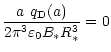
![]() is determined by the precise electrospheric
configuration around the pulsar. This can easily be seen by expressing
the condition for wind disappearance when equaling the polar line
potential at the crust given by (8) for a=0with its vanishing value at infinity. Doing this we get the optimal
charge as
is determined by the precise electrospheric
configuration around the pulsar. This can easily be seen by expressing
the condition for wind disappearance when equaling the polar line
potential at the crust given by (8) for a=0with its vanishing value at infinity. Doing this we get the optimal
charge as
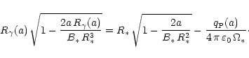
Our description is only valid if the gaps present in our solutions are
stable to charge transfer from disk to domes and to vacuum breakdown
by pair avalanches. We stressed already their stability with respect
to charge transfer. We now examine in some more detail the mechanism
of e![]() pair creation in these outer gaps and show that the
development of leptonic cascades in second pulsars with period of the
order of 1 s or so is rather unlikely and certainly unable to cause
the filling up of the magnetosphere with electron-positron plasma up
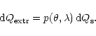
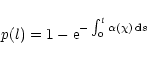
to the light cylinder. We recall that the probability p(l) of
conversion into a lepton pair of a photon of energy
pair creation in these outer gaps and show that the
development of leptonic cascades in second pulsars with period of the
order of 1 s or so is rather unlikely and certainly unable to cause
the filling up of the magnetosphere with electron-positron plasma up
to the light cylinder. We recall that the probability p(l) of
conversion into a lepton pair of a photon of energy
![]() along a
path of length l is given according to Erber (1966) by
along a
path of length l is given according to Erber (1966) by
 |
(32) |
 |
(33) |
 |
(34) |
Suppose that an electron (may be a positron) emits by curvature
radiation a photon of energy ![]() parallel to the local magnetic
field at a some place on the null surface (where magnetic field and
rotation speed are orthogonal), i.e at the position
parallel to the local magnetic
field at a some place on the null surface (where magnetic field and
rotation speed are orthogonal), i.e at the position
![]() .
When reaching a central
distance R during its trip, started at the emission point R0, the
photon sees a magnetic field
.
When reaching a central
distance R during its trip, started at the emission point R0, the
photon sees a magnetic field ![]() perpendicular to its path given
by
perpendicular to its path given
by
![]() .
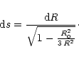
For a dipolar magnetic field, the curvilinear abscissa along the
photon path is related to the spherical radius by
.
For a dipolar magnetic field, the curvilinear abscissa along the
photon path is related to the spherical radius by
![]() .
So we get
.
So we get
| |
Figure 9:
The variation with magnetic line of the potential drop
|
| Open with DEXTER | |
| |
Figure 10:
Maximum path length before disintegration (defined by
Eq. (37)) of a photon of a given
energy |
| Open with DEXTER | |
 |
(36) |
Up to now the photon energy has been left unprecised. However we know
that the synchro-curvature radiation spectrum peaks near the frequency
![]() ,
,
![]() being the
curvature radius of the lepton's trajectory. The Lorentz factor
being the
curvature radius of the lepton's trajectory. The Lorentz factor
![]() of the emitting electron cannot exceed the electric potential
drop available in the gap on the magnetic surface on which it moves.
Then we find as an upper bound
of the emitting electron cannot exceed the electric potential
drop available in the gap on the magnetic surface on which it moves.
Then we find as an upper bound
![]() ,
,
![]() being the potential drop between one dome and the
equatorial belt along the magnetic line a, that is:
being the potential drop between one dome and the
equatorial belt along the magnetic line a, that is:
 |
(39) |
| |
Figure 11:
Optical depth |
| Open with DEXTER | |
 |
(40) |
The energy of curvature photons never exceeds that of their emitter,
which appears to be limited to approximately
![]() .
In fact
most curvature photons are much less energetic than the lepton which
emits them so that
.
In fact
most curvature photons are much less energetic than the lepton which
emits them so that
![]() .
The characteristic
curvature photon energy is given by
.
The characteristic
curvature photon energy is given by
![]() .
With
.
With
![]() we find
we find
![]() TeV.
Looking at Fig. 10, we see that for pulsars with a
magnetic field strength of B*=108 T the breakdown region is
limited to about fifty stellar radii (independently of his rotation
period). This is negligible compared to the light cylinder radius for
both P=1 s (
TeV.
Looking at Fig. 10, we see that for pulsars with a
magnetic field strength of B*=108 T the breakdown region is
limited to about fifty stellar radii (independently of his rotation
period). This is negligible compared to the light cylinder radius for
both P=1 s (
![]() )
and P=0.1 s (
)
and P=0.1 s (
![]() ). This only goes to show that curvature photon
conversion into a pair on the magnetic field is not an efficient
enough mechanism to break the vacuum gaps which appear in our
solutions. Unlike second-pulsars, millisecond-pulsars could fill their
vacuum gaps with pair plasma up to the light surface although their
magnetic field is only B*=105 T. Indeed, looking at the panel on
the right of Fig. 10, it is seen that the extension of
the vacuum breakdown zone for very energetic photons of about 0.1
to 1 TeV and more, is of the same order of magnitude magnitude as the
light cylinder radius
). This only goes to show that curvature photon
conversion into a pair on the magnetic field is not an efficient
enough mechanism to break the vacuum gaps which appear in our
solutions. Unlike second-pulsars, millisecond-pulsars could fill their
vacuum gaps with pair plasma up to the light surface although their
magnetic field is only B*=105 T. Indeed, looking at the panel on
the right of Fig. 10, it is seen that the extension of
the vacuum breakdown zone for very energetic photons of about 0.1
to 1 TeV and more, is of the same order of magnitude magnitude as the
light cylinder radius ![]() ,
about
,
about ![]() .
We conclude that
a magnetosphere entirely filled with leptonic plasma is quite possible
in this case.
.
We conclude that
a magnetosphere entirely filled with leptonic plasma is quite possible
in this case.
This statement remains true if the hard photons were to originate from
inverse Compton scattering of soft photons by ultra-relativistic
electrons or positrons rather than from curvature radiation. The
maximal energy reached by such photons is obviously less than the
total kinetic energy of the energetic electron involved in the
scattering process, the Lorentz factor of which is itself limited by
curvature radiation reaction to a value of magnitude 108. The
scattered photon energy ![]() never exceeds 100 TeV.
Consequently, according to Fig. 10, the same
conclusions as in the previous subsection hold.
never exceeds 100 TeV.
Consequently, according to Fig. 10, the same
conclusions as in the previous subsection hold.
The two-photon pair production is generally considered in outer gap models as a trigger for e-e+ cascade. Curvature gamma rays emitted by accelerated particles interact with the thermal X-ray photons from the polar caps. We show in this section that, for sufficiently low surface temperature, this process is negligible in the pulsar magnetosphere.
![\begin{figure}
\par\includegraphics[width=8.8cm,clip]{MS1831f12.eps} \end{figure}](/articles/aa/full/2002/11/aa1831/img198.gif) |
Figure 12:
Optical depth |
| Open with DEXTER | |
For convenience, in the following, the photon energy will be expressed
in units of
![]() .
The threshold energy
.
The threshold energy
![]() of the soft
X-ray photon for pair creation by collision with a photon of
energy
of the soft
X-ray photon for pair creation by collision with a photon of
energy
![]() at an angle
at an angle ![]() is then given by
is then given by
where
![]() is the electron classical
radius and
is the electron classical
radius and
![\begin{figure}
\par\includegraphics[width=12.2cm,clip]{MS1831f13.eps} \end{figure}](/articles/aa/full/2002/11/aa1831/img217.gif) |
Figure 13:
Optical depth |
| Open with DEXTER | |
 |
(47) |
 |
(48) |
The optical depth sharply increases with energy up to a certain
maximum and then decreases more slowly with increasing photon energy
(see Fig. 13). For instance, for T=106 K, the
maximal optical depth,
![]() ,
is reached for
,
is reached for
![]() .
Near the light cylinder of a
pulsar-second, this depth is 100 times less, due to the 1/R0scaling. It is then clear that no two-photon interaction takes place
for such a temperature, whatever the gamma-ray energy and its emission
location. This remains true for T=107 K, the optical depth
reaching 0.4 for
.
Near the light cylinder of a
pulsar-second, this depth is 100 times less, due to the 1/R0scaling. It is then clear that no two-photon interaction takes place
for such a temperature, whatever the gamma-ray energy and its emission
location. This remains true for T=107 K, the optical depth
reaching 0.4 for
![]() .
For T=108 K, however, the maximal optical depth reaches 24 for
.
For T=108 K, however, the maximal optical depth reaches 24 for
![]() and this process becomes important.
and this process becomes important.
Comparing the optical depths in Figs. 11 and 13, it is seen that photon-photon interaction is negligible compared to photon disintegration in the magnetic field.
![\begin{figure}
\par\includegraphics[width=11.6cm,clip]{MS1831f14.eps} \end{figure}](/articles/aa/full/2002/11/aa1831/img226.gif) |
Figure 14:
Change in the electrospheric structure for the model
|
| Open with DEXTER | |
Thus the ![]() -
-![]() interaction remains inefficient for
sufficiently low neutron star temperatures of the order of T=106 K
or T=107 K. It becomes significant for a hot stellar crust
with
interaction remains inefficient for
sufficiently low neutron star temperatures of the order of T=106 K
or T=107 K. It becomes significant for a hot stellar crust
with
![]() K and even more so for very hot ones. Such very
high temperatures are however not likely to be met. For usual surface
temperature (less than 107 K say), the process of lepton pair
creation by photon-photon collisions is dominated by the photon
interaction with the magnetic field very near the neutron star.
K and even more so for very hot ones. Such very
high temperatures are however not likely to be met. For usual surface
temperature (less than 107 K say), the process of lepton pair
creation by photon-photon collisions is dominated by the photon
interaction with the magnetic field very near the neutron star.
In the previous sections, we have shown that pair creation does not
take place very far away from the star for second-pulsars. Indeed,
given that the characteristic curvature photon energy is about a TeV,
the avalanche zone does not exceed a few tens of stellar radii
(say ![]() with B=108 T). How does this process influence the
electrospheric structure? Qualitatively, we can answer this question
as follows. As long as the gaps remain large enough to sustain a
sufficient potential drop between disc and domes to create pairs, the
equatorial belt will be filled with positrons (for aligned rotators)
and the domes with electrons. The size of the gap will gradually
diminish until the potential drop falls below the breakdown potential.
Its dimension will become negligible as compared to the stellar
radius. Thus in those regions where gaps become small, we may simply
assume that the domes and the disc are in contact at the null surface
and the corresponding magnetic surfaces are in corotation with the
star. These surfaces, where the pair-cascade occurred, are almost
entirely filled with charge-separated plasma at the Goldreich-Julian
density. The gaps become eventually inactive and the new
electrospheric structure will the be similar to the structure
calculated in the absence of pair creation, simply changing the stellar
radius R* to a new "effective'' one, almost equal to the
extension
with B=108 T). How does this process influence the
electrospheric structure? Qualitatively, we can answer this question
as follows. As long as the gaps remain large enough to sustain a
sufficient potential drop between disc and domes to create pairs, the
equatorial belt will be filled with positrons (for aligned rotators)
and the domes with electrons. The size of the gap will gradually
diminish until the potential drop falls below the breakdown potential.
Its dimension will become negligible as compared to the stellar
radius. Thus in those regions where gaps become small, we may simply
assume that the domes and the disc are in contact at the null surface
and the corresponding magnetic surfaces are in corotation with the
star. These surfaces, where the pair-cascade occurred, are almost
entirely filled with charge-separated plasma at the Goldreich-Julian
density. The gaps become eventually inactive and the new
electrospheric structure will the be similar to the structure
calculated in the absence of pair creation, simply changing the stellar
radius R* to a new "effective'' one, almost equal to the
extension ![]() of the avalanche zone. From an electrical point of
view, there is no distinction between the star and the corotating
electrosphere. The parameter
of the avalanche zone. From an electrical point of
view, there is no distinction between the star and the corotating
electrosphere. The parameter ![]() is but a scale factor which
defines the radius of the electrically equivalent star.
is but a scale factor which
defines the radius of the electrically equivalent star.
This remark is illustrated in Fig. 14.
Starting
with the model with a total charge
![]() shown in
Fig. 3, we have added an arbitrary source
of e-e+ defined in the interval
shown in
Fig. 3, we have added an arbitrary source
of e-e+ defined in the interval
![]() by
by
Negative surface charge remains on the crust. The algorithm in fact could not converge. This is because the equilibrium state of Fig. 14 is not self-consistently determined due to the presence of pair sources. If the pair cascade were to be stopped, charge would move back to the electrosphere to annihilate positive particles located in the disc restauring the situation described in Sect. 4. To maintain some marginal activity in the vacuum gaps, it would be necessary to allow particles to somehow escape from the system (via the equatorial plane and the poles) setting up an electric circuit. Describing this regime is the subject of our next papers.
In this paper the existence and viability of self-consistent pulsar
electrospheres, finite in extent and in electrostatic equilibrium,
have been proved in the case of aligned rotators. Large vacuum gaps
separate the corotating polar regions from a differentially rotating
belt. Compared with similar previous investigations by
Krause-Polstorff & Michel (1985b), we obtain more extended
and much better results, overcoming their problem of an empty cone
about the polar axis due to the artifact of the quantization of the
surface charge. Moreover the shape of the electrosphere is in our
case well defined, allowing us to obtain smooth rotation curves
without any more noise than allowed by roundoff errors. We have also
investigated the effect of charge loss from the polar caps and we have
shown that it self-saturates in the absence of return current
precisely by developing a charged electrostatic dome above them, as
pictured by the entirely electrostatic model. Therefore the system is
unlikely to evolve to a state where it emits a wind with no net charge
loss.
Contrary to what is generally believed, the vacuum breakdown of these
large gaps by e![]() pair creation is not efficient enough to cause
the filling-up of the whole magnetosphere up to the light surface by
leptonic plasma. This statement unambiguously holds true for pulsars
with periods in the range of a second. For the class of millisecond
pulsars the conclusion remains unclear and would require a more
precise evaluation of pair-creation effects as well as a relativistic
description of the electrosphere.
pair creation is not efficient enough to cause
the filling-up of the whole magnetosphere up to the light surface by
leptonic plasma. This statement unambiguously holds true for pulsars
with periods in the range of a second. For the class of millisecond
pulsars the conclusion remains unclear and would require a more
precise evaluation of pair-creation effects as well as a relativistic
description of the electrosphere.
There is however more to the structure of such electrospheres than just their axisymmetric equilibrium properties. The existence of a differentially rotating disk opens up the question of the stability of the plasma in such a configuration. This will be the purpose of a future paper where this question will be studied. It will be shown that the plasma is indeed most often unstable to the so called diocotron instability and the consequences of this situation will be studied.
At the stellar surface the potential equals the corotation one and in
the nearby vacuum, if any, it satisfies Laplace equation, the general
solution of which can be expressed as
 |
(A.1) |
| |
= |  |
|
 |
(A.2) |
| |
= | ||
![$\displaystyle -\frac{1}{5}\,\left[ \frac{2}{3}\Omega_\ast\,B_\ast\,R^2
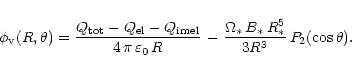
+ \frac{\Omega_\ast\,B_\ast\,R_\ast^5}{R^3} \right] \, P_2(\cos\theta).$](/articles/aa/full/2002/11/aa1831/img244.gif) |
(A.4) |
| |
= | ![$\displaystyle \frac{Q_{\rm c}}{4\,\pi\,\varepsilon_0\,R^2}
\, \vec{e}_{\rm R} %...
...\Omega_\ast\,B_\ast\,R
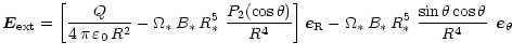
- 3 \frac{\Omega_\ast\,B_\ast\,R_\ast^5}{R^4} \right] \,$](/articles/aa/full/2002/11/aa1831/img247.gif) |
|
![$\displaystyle \times \left[ \frac{2}{3}\Omega_\ast\,B_\ast\,R
+ \frac{\Omega_\ast\,B_\ast\,R_\ast^5}{R^4} \right] \, \vec{e}_\theta.$](/articles/aa/full/2002/11/aa1831/img249.gif) |
(A.5) |
 |
(B.3) | ||
 |
(B.4) | ||
 |
(B.5) |


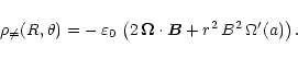
![$\displaystyle \left[ f(R)+ \frac{R\,\sin\theta}{2}\,\frac{{\rm d}f}{{\rm d}R} \right]
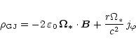
\,\rho_{\rm GJ}.$](/articles/aa/full/2002/11/aa1831/img130.gif)
![\begin{displaymath}\,\,\,\,\,\,\,\,\,\,\,\,\,\,\,\,\,\,\,\,\,\,\,\,\,\,\, - \,2\,\beta\,\big(2
-\beta^2\big) \bigg]
\end{displaymath}](/articles/aa/full/2002/11/aa1831/img210.gif)

![$\displaystyle { \vec{e}_{\rm B} \cdot \vec{E} = - \frac{3}{5}\sin^2\theta\cos\t...
..._\ast\,R
+ \frac{\Omega_\ast\,B_\ast\,R_\ast^5}{R^4} \right]\!
+ 2 \cos\theta
}$](/articles/aa/full/2002/11/aa1831/img250.gif)
![$\displaystyle \times \left[ \frac{Q_{\rm c}}{4\,\pi\,\varepsilon_0\,R^2}
+ \fra...
...ft( \frac{4}{3} R
- 3 \frac{R_\ast^5}{R^4} \right) P_2(\cos\theta) \right]\cdot$](/articles/aa/full/2002/11/aa1831/img251.gif)