A&A 383, 227-238 (2002)
DOI: 10.1051/0004-6361:20011739

Automated spectroscopic abundances of A and F-type stars
using echelle spectrographs

I. Reduction of ELODIE spectra and method of abundance determination

D. Erspamer - P. North

Institut d'astronomie de l'Université de Lausanne, 1290 Chavannes-des-Bois, Switzerland

Received 11 October 2001 / Accepted 12 November 2001

Abstract
This paper presents an automated method to determine detailed abundances for A and F-type stars. This method is applied on spectra taken with the ELODIE spectrograph. Since the standard reduction procedure of ELODIE is optimized to obtain accurate radial velocities but not abundances, we present a more appropriate reduction procedure based on IRAF. We describe an improvement of the method of Hill & Landstreet (1993) for obtaining $V\sin{i}$, microturbulence and abundances by fitting a synthetic spectrum to the observed one. In particular, the method of minimization is presented and tested with Vega and the Sun. We show that it is possible, in the case of the Sun, to recover the abundances of 27 elements well within 0.1 dex of the commonly accepted values.

Key words: methods: numerical - techniques: spectroscopic - Sun: abundances - stars: abundances - stars: individual: Vega

1 Introduction

The determination of detailed abundances requires a high resolving power (>$30\,000$) and a wide spectral range. In order to satisfy both requirements simultaneously, echelle spectrographs must be used. ELODIE (Baranne et al. 1996, hereafter BQ96) is a fiber-fed echelle spectrograph with a resolution of $R=42\,000$ attached to the 1.93m telescope of the Observatoire de Haute-Provence (OHP), France. This spectrograph and its reduction software were optimized to measure accurate radial velocities.

In this paper we first show what precautions have to be taken to use ELODIE for other spectroscopic analyses, in our case detailed abundance determinations. To achieve our goal we had to make another reduction, starting from the raw image and taking special care in the removal of scattered light. Another important point in the reduction is to paste together the different orders of the spectrum and normalize them. Secondly, we present a method to estimate abundances with synthetic spectra adjustments. This method is an improvement of that of Hill & Landstreet (1993, HL93 hereafter). It is automated as much as possible and is able to analyse stars with various rotational velocities (up to 150  ${\rm km~s^{-1}}$), for which the equivalent width method is not applicable. Finally, to assess the validity of this method, we compare the abundances derived for Vega ($\alpha$ Lyr = HR 7001 = HD 172167) and the Sun with those in the literature. These two reference stars are used to check the code's validity for stars having effective temperatures between those of the Sun and of Vega.

Analysis tools with related goals but different approaches have been developed by Valenti & Piskunov (1996), Cowley (1996) and Takeda (1995a). Takeda's method has been used by Varenne & Monier (1999) to derive abundances of A and F-type stars in the Hyades open cluster.

  
2 Observations

The spectra used in this work were obtained with the ELODIE echelle spectrograph (see BQ96 for technical details) attached to the 1.93m telescope of the Observatoire de Haute-Provence (France) during August 1999. A high S/N (>300) spectrum of Vega was obtained covering the range of 3900-6820 Å.

The best way to check both reduction and analysis is to obtain a good quality solar spectrum with ELODIE, in the same conditions as in the case of stellar observations. The target can be either an asteroid or one of the Jovian moons in order to have a point-like, but bright enough source. Our choice was Callisto, and it was observed on 13 August 1999 when it was almost at a maximum angular distance from Jupiter, thus avoiding light pollution by the planet. The resulting spectrum has a S/N of about 220 at 5550 Å.

3 Data reduction

The primary goal of the ELODIE spectrograph was to measure high-accuracy radial velocities, and the data reduction pipeline was optimized for that purpose. The on-line reduction is achieved by the software INTER-TACOS (INTERpreter for the Treatment, the Analysis and the COrrelation of Spectra) developed by D. Queloz and L. Weber at Geneva Observatory (BQ96). During this reduction, the background is removed using a two dimensional polynomial fit that has a typical error of about 5%, with a peak in the middle of the orders (cf. Fig. 11 of BQ96). We tried to improve this fit by increasing the polynomial order. However, we encountered an internal dimensional limitation that prevented us from using a high enough order to correct the middle peak. Therefore, we decided to use IRAF (Image Reduction and Analysis Facility, Tody, 1993 ). Another point motivating our choice was the wide availability of IRAF.

3.1 Overview of the reduction procedure

The reduction itself was done with IRAF, and more precisely with the imred.ccdred and imred.echelle package. Its main stages are the following:

• Combination and averages of the calibration exposures (offsets, darks, "flat-fields") with the IRAF functions zerocombine, darkcombine and flatcombine;
• Correction of the object exposure from the offset, dark and bad pixels, taking into account the overscan level with ccdproc;
• Finding, centering, resizing (i.e. function that estimates the width of the orders), and tracing the orders using the flat image with apfind, apcenter, apresize, aptrace;
• Removal of the diffuse light of all raw images except the wavelength calibration one with apscatter;
• Recentering, resizing, retracing and extracting the flat-field spectrum with apsum;
• Extraction and calibration of the thorium image with apsum, ecidentify, ecreidentify;
• Extraction of the object spectra using the variance weighting method (Horne 1986) with apsum;
• Division by the extracted flat-field spectrum with sarith;
• Wavelength calibration of the object spectra with dispcor;
• Merging the 67 orders with a home-made fortran program to obtain one spectrum for the whole range of ELODIE;
• Normalization to the continuum using the IRAF continuum function.

3.2 Removal of scattered light

The main weakness of the online procedure resides in the background subtraction. Although a typical error in the background measurement of 5% can be tolerated for accurate radial velocity measurements (BQ96), it is important to achieve a better adjustment in order to use the spectra for abundance measurements. The scattered light is estimated, smoothed and subtracted in the following way. Interorder pixels are fit with a one dimensional function in the direction perpendicular to the dispersion. This fitting uses an iterative algorithm to further reject high values and thus fits the minima between the spectra. The fitted function is a combination of 30 spline functions (see Fig. 1 Top). Because each fit (each column) is done independently, the scattered light thus determined will then be smoothed by again fitting a one dimensional function (30 spline functions in the dispersion direction). The final scattered light surface is then subtracted from the input image. The reason for using two one-dimensional fits as opposed to a surface fit is that the shape of the scattered light is generally not easily modeled by a simple two dimensional function. The typical error in the background measurement is about 2%. This is shown in Fig. 1, which should be compared with Fig. 11 of BQ96.

It is to be noted that the blue orders are not very well corrected. However, this is a deliberate choice. We cannot simultaneously adjust the first orders without using more than 35 cubic spline functions. But with that number, the fitting function is too sensitive to the order. Moreove, since the signal to noise ratio (S/N) is lower in the bluest orders (see Fig. 10 of BQ96), these are not optimal for abundance determination. In these orders, it is very difficult to adjust the continuum because of the calcium and Balmer lines. Therefore, we decided not to use the first orders and the problem of the background subtraction in them was left unresolved.

3.3 Minor changes

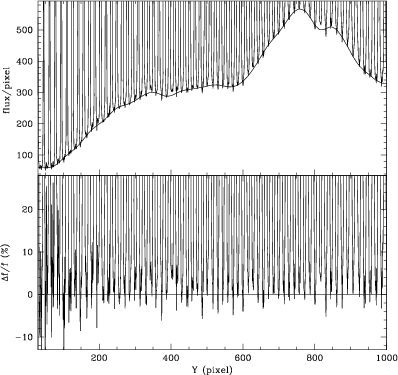	Figure 1: Top: cross order tracing at X=512 of a localization exposure superimposed with the fit of the background. Bottom: difference between the fit and the background level $\Delta f/f = (f_{\rm image} - f_{\rm fit})/f_{\rm fit}$. The typical error in the background measurement is below 2%.
Open with DEXTER

During the observing run every night, we did many offsets, darks and flat-fields. Instead of using only the last exposure for the offset, dark and flat-field correction, as is the case in the online reduction, we chose to combine the exposures in order to remove pixels hit by cosmic rays, and obtain a mean offset, dark and flat-field. Then we corrected each pixel of the object image with the corresponding one of the offset and dark.

Then we used the average flat-field (while the standard TACOS reduction only uses the last one) to determine the shape of the orders and this shape was used as reference for the extraction of the object image. We took care to adjust the resizing parameter with the lowest possible parameters in order to get almost all the flux. Finally, we set the aperture limit at 0.005 time the level of the peak. This lead to the extraction of 99.9% of the flux spread over the order.

As explained in the paper BQ96, the flat-field spectrum correction method (i.e. flat-field correction after extraction of the spectrum) is satisfactory with such a stable instrument as ELODIE. This method is also applied in our reduction (in any case, it is not really possible to get a true flat-field image with ELODIE).

The wavelength calibration is carried out using the thorium spectrum. The spectra are extracted without correction of the scattered light and without the flat-field division. A two dimensional Chebyshev polynomial is used to constrain the global wavelength position with the degree 7 for both directions. The typical rms between the fit and the location of the lines is always below 0.001 Å for the wavelength calibration of the whole spectrum. The fit is just a formal one. We did not attempt to model the optical behaviour of the spectrograph. We used the thar.dat file from IRAF to identify the lines. This file contain the line list of a Thorium-Argon spectral Atlas done by Willmarth and collaborators available at http://www.noao.edu/kpno/specatlas/thar/ thar.html which used identification from Palmer and Engleman (1983, the same as BQ96) for Th and from Norlén (1976) for Ar. Looking carefully at the flux ratio in Fig. 5, bottom, a number of the larger discrepancies appear to be due to minute wavelength differences between both spectra. A difference of $50\,{\rm m~s^{-1}}$ might already explain such a signature in the ratio panel. Figure 14 of BQ96 shows that the accuracy differs from one order to the other. Figure 5 displays more than two orders, and differences appear only in the left and right parts, which correspond to different orders than the central part. As accuracies are different, it is possible that small shifts exist between orders.

3.4 Merging the orders

	Figure 2: 19th, 20th and 21th orders of Vega before merging.
Open with DEXTER

The next important task is to merge the orders to obtain a one dimensional spectrum covering the whole wavelength domain. At that point, we encountered a problem with the data. The extracted orders are not flat enough to be merged using the average or median value of the order as coefficient (see Fig. 2).

Merging by considering only one average value per order results in a spectrum with steps (imagine Fig. 2 with a vertical line connecting the middle of the overlapping region, and smooth that transition region over 10 pixels).

	Figure 3: The whole spectrum of Vega.
Open with DEXTER

We decided to compute our own program to paste the orders. There is an overlapping region until the 64th order. However the overlapping region is large enough to estimate the ratio only until the 50th order. (Note that the orders are numbered from 1 to 67 and the "true'' number in not used as in BQ96). Therefore, we used two different merging methods, one using the overlapping region for the orders 1 to 50, and another using the first and last 200 points of the order (each order is rebinned with a step of 0.03 Å before the merging). With both methods, we computed a ratio allowing to scale the orders, starting from the middle order which is used as reference.

In the first method, we computed the average of the ratios of the overlapping points and the rms scatter. Then, we did a loop taking into account only the ratios between the average $\pm 2 \sigma_{\rm rms}$ until no points were deleted or the number of points become $\leq$50. This method was very efficient, and worked in almost every case.

The second method was not quite as efficient but we rarely had to correct its results manually. We decided to use the first and last 200 points of the orders, compute the average value of these points and the rms scatter, then recompute the average but deleting the points that were not between the average $\pm 2 \sigma_{\rm rms}$ until no points were deleted or the number of points became $\leq$50 and finally compute the ratio of the averages of the end of an order and the beggining of the following order.

Finally, starting from the middle order, the orders are scaled by multiplicative adjustments. In the overlapping regions, no attempt was made to make a weighted average: in view of the blaze function, it was decided to retain the flux of the first order for 3/4 of the overlapping region and the flux of the following order for the remaining 1/4. Both methods are compatible and it is possible to merge all orders in a single pass; Fig. 3 shows the results for Vega.

3.5 Normalization

	Figure 4: Plot of the 31th order of Vega around H$\beta$.
Open with DEXTER

The final step is normalization to the continuum level. A simple look at Fig. 3 shows that it is no easy task, especially around the Balmer lines H$\alpha$ and H$\delta$ and the Caii K line. We decided to use the function continuum of IRAF. However, it is very hard to normalize the whole spectrum in a row. One could argue that, if the normalization was done before merging, that operation would become much easier. However, some orders are not normalizable, especially those containing the Balmer lines (see Fig. 4).

We chose to split the whole spectrum into 6 parts, and normalize each part separately (besides analyzing the whole spectrum at once would require too much data processing). The task continuum has many parameters and the result is very dependent on them. However, once a good set of parameter is defined, it can be used for a lot of different spectra. Moreover, IRAF allows to modify the parameters interactively in case of unexpected behaviour.

Although IRAF works well automatically, it is important to check all the spectra visually. Unfortunately, despite all different numerical tests, the eyes appear to be still the best way to decide which set of parameters to use.

3.6 Check with a reference spectrum

	Figure 5: Top: solar spectrum extracted with the optimized IRAF reduction. Middle: ratio between the spectrum resulting from the standard TACOS procedure and the solar spectrum from Kurucz. Bottom: ratio between the spectrum resulting from the optimized IRAF reduction and the solar spectrum from Kurucz.
Open with DEXTER

Our reduction was checked using the Solar Atlas from Kurucz et al. (1984). This spectrum was acquired with a very high resolving power ($300\,000$) and a very high signal to noise ratio (3000). The resolving power was adjusted to that of ELODIE by convolving the spectrum with an instrumental profile; a simple Gaussian with an FWHM corresponding to the normal resolution $R=42\,000$ was considered sufficient. Our comparison spectrum was acquired using Callisto so that we were in a stellar-like configuration. This precaution is not very important as ELODIE is a fiber-fed spectrograph, but one of the advantages was that it required a rather long exposure and therefore the reduction was sensitive to the dark correction. Finally, we adjusted the radial velocities. Notice that two versions of the spectrum, one resulting from the TACOS reduction procedure and the other from the IRAF procedure, were merged and normalized using our method. The comparison is illustrated in Fig. 5.

It is clear, looking at the ratio for the strong lines, that scattered light is not well subtracted with the standard TACOS procedure. The difference increases as lines strengthen, reaching a maximum at the core of H$\beta$ in our example. Even if the difference for H$\beta$ can partly come from the normalization as can be seen looking at the ratio in the wings, which differ slightly from 1, the big difference in the core cannot be assigned to different continuum adjustment. On the contrary, our optimized reduction leads to differences which remain within, or only slightly larger than the noise.

4 Abundance analysis

This section presents the method for abundance analysis. In the first part (Sect. 4.1), the spectrum synthesis program is described. In the second (Sect. 4.2), the minimization method is explained.

This method adjusts the abundances using synthetic spectra. The starting point was the program described in Hill & Landstreet (1993), which was used to determine detailed abundances in A-type stars and has been kindly provided by Dr. G. M. Hill. The modifications made to this program will be presented in this section.

  
4.1 spectrum synthesis

The spectral synthesis code used here is similar to the one described in HL93. It is an LTE synthesis code (see HL93 for details). Various modifications were done:

• The code from HL93 used the model atmospheres ATLAS5 of Kurucz (1979). It was modified to allow the use of ATLAS9 models. However, the format of the models has changed. In ATLAS5, there was a column containing the geometrical depth X and another containing the optical depth at 5000 Å, $\tau_{5000}$, and the code of HL93 uses it to compute the optical depth at each wavelength of the spectrum ( $\tau_{\lambda}$). However, in ATLAS9 the depth is only given in the "rhox'' parameter which is the density integrated as far as the geometrical depth X. In order to modify the code as little as possible, we only changed the way $\tau_{\lambda}$ is computed. A subroutine of the ADRS code (Y. Chmielewski 2000) was used to reformat the model as a function of $\tau_{5000}$. Then it was easy to use $\tau_{5000}$ instead of X and the following equation was used for the calculation of the optical depth at each wavelength step.
  
  $$\tau_{\lambda} = \int{\frac{\kappa_{\lambda}}{\kappa_{5000}} {\rm d}\tau_{5000}}$$
  
  
  ATLAS9 was installed on a SunBlade100 computer (Sun UltraSparcII machine). The Unix version adapted by M. Lemke was used because the version of Kurucz (1993) is adapted to VAX-VMS. It will allow to compute models with the right effective temperature, gravity, metallicity and microturbulent velocity. Models will be computed without overshooting as it appears that they are best adapted to abundances analysis (see for example Castelli et al. 1996);

• The second modification allows the use of the VALD database (Piskunov et al. 1995, Kupka et al. 1999 and Ryabchikova et al. 1999 ) as the source of line list parameters. This database provides $\gamma_4 / N_{\rm e}$ and $\gamma_6 / N_{\rm H}$ at 10000 K for the Stark and van der Waals damping parameters respectively instead of C₄ and C₆ used by HL93. In case these values are not available, the damping parameters are calculated using the formulae described in HL93;

• The polynomial partition functions were completed for as many elements as possible, using data from Irwin (1981) and Sauval & Tatum (1984). In case that the function is unavailable, the program uses the statistical weight of the lowest energy level. However, for some elements like Co and Ba, using a partition function or the approximate value may result in abundance changes as high as 0.2 dex;

• Finally, there were several other changes, including the introduction of dynamical memory allocation. However, the theoretical assumptions used in the initial code do not change.

  
4.2 Abundances determination

  
4.2.1 Line list

Instead of using a set of meticulously selected lines, the first hope was to use the line list as it comes from the VALD database, using the "extract stellar'' option. This choice was motivated by the large spectral range of ELODIE. The idea was to use a large number of lines with parameters not necessarily well known, but considering a large number, the effect of poor $\log{gf}$ should disappear and the mean value for an element should be correct. This idea is justified for elements of the iron peak, but not for elements as Si, Sr, Ba, and heavier elements. For these elements (except for Si), only one or a few lines are present, and it is easy to understand that if there are only a few lines, the abundance is very sensitive to the line parameters.

Although VALD-2 provides the most recent collection of oscillator strength data, it appears that for some elements with few lines (and Si), the $\log{gf}$ values had to be examined individually and adjusted whenever possible (i.e. when the line was not blended). To achieve good adjustment, lines of problematic elements were checked individually and 2 methods were used to adjust the oscillator strength using the Sun spectrum:

• The line was checked for presence in the line list coming from the SPECTRUM package of Gray (1994, and available at http://www.phys.appstate.edu/spectrum/spectrum.html) that contains adjusted $\log{gf}$ for some lines. If such was the case, and if the value was different, this value was tried. Then if it gave good results it was retained;

• In case of failure of the first method, the value was adjusted on the Solar spectrum with an iterative procedure until the abundance was correct within 0.05 dex.

Finally, instead of using directly the VALD result, a reference line list covering our spectral domain was compiled, and used for all the stars to be analyzed. It is to be noticed that this line list may still contain erroneous $\log{gf}$ values because every line is not necessarily visible in the solar spectrum, and also because this parameter was only adjusted for problematic elements when the line was clearly identifiable. Moreover, lines can be individually erroneous, but when all lines of an element are used together, the individual errors seems to cancel out. This is the case in particular for iron where statistically, the abundance is correct while a lot of lines have inaccurate $\log{gf}$ values. For other elements, it is not obvious that these errors should average, but the application of the method for the Sun seems to indicate that it is the case (see Sect. 5.3).

4.2.2 Minimization method

The program of HL93 uses the technique known as "downhill simplex method''. This method is certainly the best if the goal is "to get something working quickly'', in the sense that it does not have strong initial constraints. Another advantage is that it does not require derivatives. However, it is not the fastest one. Moreover, in our case, the function to be evaluated requires computation of a synthetic spectrum. The major improvement in time will come from lowering the number of spectra to be computed. Looking for minimization methods of multidimensional functions in "Numerical Recipes'' (Press et al. 1992), we decided to implement a direction set method in multidimensions known as Powell's method. This method can be summarized as follows. Given a set of N directions (where N is the number of free variables), the method performs a quadratic minimization along each direction and tries to define a new one as the direction of the largest decrease. We simply adapt the Numerical Recipies code by adding some tests to avoid looping that may occur if the program tries to adjust lines of an element that are too faint to be of any significance.

Initial conditions: in order to use this method an initial set of directions has to be defined. The goal is to adjust radial, rotational and microturbulent velocities as well as abundances. In order to be efficient even in the first iteration, it appears that the best choice of directions is to adjust successively radial velocity (which is fixed when it is available from ELODIE online reduction), rotational velocity, the abundances starting from the element with the maximum of significant lines, and finally microturbulent velocity. As we do not know a priori the abundance pattern, the starting point is the solar one. Note that the solar abundances will always refer to Grevesse & Sauval (1998). The order proposed is justified by the following example. Let us consider a blend of two lines of different elements; the element with the largest number of lines will be adjusted first. As it has other lines, it is less sensitive to the blend and the program does not try to fill the blend by increasing the abundance of this element only, as it would happen if the element with only one or two lines was adjusted first. Then the second element is adjusted in order to fill up the blend.

Procedure of analysis: it is important to retain only the lines from the reference list that contribute to the spectrum. Therefore lines were sorted using the equivalent width computed with a reduced version of the program. Only lines with an equivalent width larger than 10 mÅ (when computed with an atmosphere model corresponding to the stellar parameters and solar abundances) are used for the first abundance determination. The results of this first minimization are used to re-sort out the lines with the same equivalent width criterion. Then a second computation is done with the new line list, using the result of the first computation as a starting point for the velocities and abundances. That speeds up the second adjustment.

This analysing procedure allows to eliminate a lot of lines that are significant for solar abundances but are no longer visible when it comes to abundances of the star. Conversely, it may also allow to gain lines that were too weak for solar abundances but are strong enough with the stellar value.

Speed optimization: during abundance analysis, a synthetic spectrum is computed at each step of the minimization procedure. It is important to find a way to reduce the time of analysis as much as possible.

The spectral range of ELODIE is wide (3900-6820 Å). In order to have the best possible abundance estimates, it is important to use the largest number of lines i.e. the widest possible spectral range. However it is not possible, with this method, to use the whole spectral range at once for various reasons:

• The program does not implement the computation of Balmer lines because HL93 only used small spectral windows. It only implements H$\beta$ but this line is just treated as a correction to the continuum. The other Balmer lines are not computed. Only H$\beta$ was included by HL93 because the HeI $\lambda4922$ line lies in its red wing, and it was an important line for the stars they studied;

• Running the program on a spectrum from 5000 to 6500 is much slower than adjusting 4 parts of 400 Å successively on the same computer. This is surprising, but may come from inadequate programming as would be the case if looping in an array using the bad order of indices (one index is going much faster than another);

• The memory used by the program has to be kept within reasonable values because it is important to be able to dispatch the task on a large number of computers as the sample of stars to study is large. However if the required memory is too large, the use of a given computer is no longer possible or the program has to be stopped during working hours;

• Because of the strong lines of hydrogen and calcium and the resulting shape of the spectrum in the range 3900 to 4100 Å(see Fig. 3), it is very difficult to define the continuum there. The difficulty is enhanced by the small efficiency of ELODIE in the blue.

Therefore the spectra were cut in the 7 parts defined in Table 1.

   

Table 1: Definition of the 7 parts in Å.

spectral range

4125-4300

4400-4800

4950-5300

5300-5700

5700-6100

6100-6500

6580-6820

	Figure 6: Top: superposition of a part of the observed spectrum (thin line) and the synthetic one (thick line) for Vega. The atomic numbers and ionization stages (1 for singly ionized) of the species are indicated under the lines. Bottom: ratio synthetic to observed.
Open with DEXTER

Working with 7 parts, however, implies that we have 7 different estimates for each abundance. The final abundance is obtained by a weighted mean of the 7 individual estimates. Each individual value is weighted by the number of lines having a synthetic equivalent width larger than 10 mÅ.

It is important to note that telluric lines were not corrected for before analysis. Two of the seven parts contain a large number of these lines. They are the two parts going from 5700 to 6500 Å. It appears that given the width of the parts, there are enough lines for each element so that the minimization routine is not misled by the telluric lines. The exception may come in some slowly rotating stars from elements with only one or two lines which are well superposed with telluric lines.

Finally, it appears that this method is much more efficient than the downhill simplex one when it comes to adjust abundances of element with only a few lines. In the first iteration, the abundance of each element is adjusted in turn even if the $\chi^2$ value does not change a lot, whereas with the downhill simplex method, a step in the direction of an element with only a few lines is unlikely. Moreover, it takes less computer time. One reason is that a test was added to the minimization routine so that an element, the abundance of which does not change by more than 0.1% in two successive iterations, is no longer adjusted.

5 Validation

To ensure that this program would work with our sample of A-F type stars, synthetic, Vega and solar spectra were used.

  
5.1 Comparison with another spectrum synthesis code

  

Table 2: Abundance determination for a synthetic spectrum computed with SYNSPEC and known abundances.

$${ \begin{tabular}{c r @{.}l r @{.} l} \hline Element & \mul... ...$-$6&01\\ Ni & $-$5 & 89 & $-$5&91\\ \hline \end{tabular}}$$

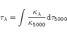
In order to check the modifications of the spectral synthesis part, a spectrum was produced using SYNSPEC (Hubeny et al. 1994) with a given model ( $T_{\rm eff} = 7500~{\rm K}$, $\log{g} = 4.0$), line list, abundances, radial and rotational velocities (see Table 2). The same input parameters were used to produce a spectrum with our code. Both codes give almost the same spectrum as can be judged by eye when looking at the ratio of both spectra. That validated the spectrum synthesis part.

In order to check the minimization routine, the spectrum from SYNSPEC was used as the one to be analyzed. Since the routine needs a starting point, solar abundances were used.

The agreement between the input and converged abundances is very good (see Table 2). The difference is always $\leq$0.03 dex. Moreover, all velocities ( $V_{\rm rad}, V\sin{i}, \xi_{\rm micro}$) were very well adjusted, even starting from very different values.

  
5.2 Vega

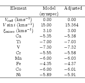
G.M. Hill provided us with a spectrum of Vega going from 4460 to 4530 Å, that was used to debug the modifications of the code. Then a spectrum was obtained with ELODIE. As there were a lot of changes, it is no longer possible to reproduce the abundances exactly as Hill's original program, essentially because of the change of the model atmosphere and lines list sources. However, the abundances estimated after the modifications are in agreement with the ones of HL93 within 0.2 dex except for Y where only one line was used.

For Vega, we used the model computed especially for this star by Kurucz and available on his web page http://cfaku5.harvard.edu/. This model is computed without convection and with stellar parameters as follows: $T_{\rm eff}=9400$K, $\log{g}=3.90$ and $\xi_{\rm micro}=0~{\rm km\,s^{-1}}$.

The whole procedure was run on the ELODIE spectrum and the results are given in Table 3.

   

Table 3: Derived abundances ( $\log{\left[\frac{N}{N_{\rm H}}\right]}$) and velocities $({\rm km\,s^{-1}})$ for Vega compared with works of HL93, Adelman & Gulliver (1990), Lemke (1989, 1990 and references therein), and Qiu et al. (2001).

Elt	Abund	HL93	Adelman	Lemke	Qiu
He	-1.36	-1.20	-1.52
C	-3.51	-3.53		-3.51	-3.54
O	-3.34				-2.99
Na	-5.69	<-5.1			-5.55
Mg	-4.84	-4.69	-5.09		-5.27
Si	-5.11	-5.14		-5.06	-5.04
Ca	-6.10	-6.11	-6.21	-6.18	-6.67
Sc	-9.58		-9.62		-9.67
Ti	-7.55	-7.36	-7.47	-7.50	-7.42
Cr	-6.91	-6.81	-6.76		-6.81
Fe	-5.14	-5.03	-5.08	-5.03	-5.07
Sr	-10.03	<-7.6		-9.93	-10.72
Y	-9.96	-10.38			-10.35
Ba	-10.51	-10.51	-10.58	-10.57	-11.19
$T_{\rm eff}$	9400	9560	9400	9500	9430
$\log{g}$	3.90	4.05	4.03	3.90	3.95
$V_{\rm rad}$	-13.25	-13.1	-13.26
$V\sin{i}$	23.2	22.4	22.4
$\xi_{\rm micro}$	1.9	1.0	0.6	2.0	1.5

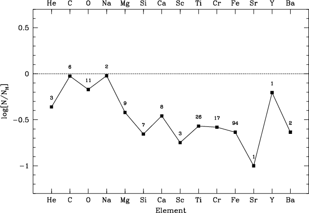	Figure 7: Logarithmic abundances of Vega with respect to the Sun. The numbers indicate the numbers of lines with an equivalent width bigger that 10 mÅ.
Open with DEXTER

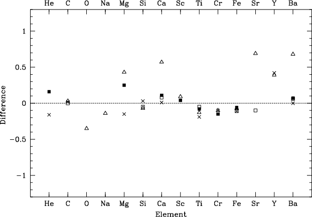	Figure 8: Difference for Vega between this paper and different authors ($\times$ HL93, $\blacksquare$ Adelman, $\square$ Lemke, and $\vartriangle$ Qiu).
Open with DEXTER

Our estimates are in good agreement with the values available from the literature (see Fig. 8 and Table 3). However, it is difficult to compare the abundance pattern for Vega directly because of the differences in the choice of fundamental parameters (see Table 3). For this star, a difference of some tenths of dex is not surprising. These differences are the main problem when it comes to compare results from different authors. Moreover, for some elements, only a few lines (sometimes only one, see number in Fig. 7) are available and it implies that these elements are much more sensitive to errors on the line parameters such as $\log{gf}$. Finally, in Vega, NLTE effects are not negligible for some elements. For example, a correction of 0.29 dex for barium was calculated by Gigas (1988). This paper is limited to LTE analysis, but it will be important to check for NLTE effects when looking for trends in element abundances.

  
5.3 The Sun

Even if it is not easy to compare studies of various authors on Vega, it has the advantage to be easy to observe and it is one of the "standard'' A0 stars even though it is underabundant. Moreover, the original spectrum synthesis code was intended for A-type stars so it is important to check its validity for cooler stars since we want to use it on F-type stars too. Therefore in order to carry out a much stronger comparison, a solar spectrum was used (see Sect. 2 for observation details). The solar spectrum is much more crowded than the Vega one. It is not always easy to find continuum points, and the abundance that will be determined will show not only whether our minimization method is efficient but also how well the continuum was placed. In any case, a careful comparison with the Solar Atlas was done on the whole spectral range. Figure 5 shows an example of the comparison on a small spectral range.

For the Sun, we computed a model with solar parameters ( $T_{\rm eff}=5777$ K, $\log{g}=4.44$ and $\xi_{\rm micro}=1~{\rm km\,s^{-1}}$) without overshooting.

As explained in Sect. 4.2.1, it was necessary to adjust some $\log{gf}$ values in order to get "canonical'' solar values for some elements. The biggest problem was with Si. A lot of its lines turned out to have intensities very different from the ones observed when computed with VALD $\log{gf}$ (for Vega, the only useful Si lines had correct gf values). Moreover, the errors were very important and could not come from a wrong placement of the continuum. One can wonder why the estimated Si abundance differs by more than 0.05 dex from the canonical one, while $\log{gf}$ values were adjusted. In fact, we tried to adjust as few lines as possible. It is always possible that small differences between observed and synthesized spectra result from unresolved lines or weak lines that are not in the line list and therefore not computed. A special care was brought in the computation of lines that were not strong enough in the computed spectrum to check how far a sum of weak lines might explain the gap. An interrogation of VALD around such lines was done, showing that the difference was never coming from forgotten lines.

	Figure 9: Top: superposition of a part of the observed spectrum (thin line) and the synthetic one (thick line) for the Sun. Bottom: ratio synthetic to observed.
Open with DEXTER

   

Table 4: Derived abundances for the Sun, difference with values from Grevesse & Sauval (1998) and number of lines with an equivalent width bigger than 10 mÅ.

Elt	Abundance	difference	# lines
	$\log{\left[\frac{N}{N_{\rm H}}\right]}+12$
C	8.56	0.04	3
Na	6.31	-0.02	18
Mg	7.52	-0.06	22
Al	6.42	-0.05	6
Si	7.48	-0.07	76
S	7.22	-0.11	3
Ca	6.34	-0.02	69
Sc	3.18	0.01	26
Ti	5.01	-0.01	361
V	4.04	0.04	87
Cr	5.71	0.04	368
Mn	5.49	0.10	81
Fe	7.52	0.02	1507
Co	4.91	-0.01	84
Ni	6.22	-0.03	292
Cu	4.23	0.02	5
Zn	4.69	0.09	3
Ga	2.84	-0.04	1
Sr	2.95	0.02	3
Y	2.20	-0.04	20
Zr	2.67	0.07	19
Ba	2.15	0.02	7
La	1.16	-0.01	5
Ce	1.66	0.08	20
Nd	1.56	0.06	12
Sm	1.08	0.07	3
Eu	0.55	0.04	2

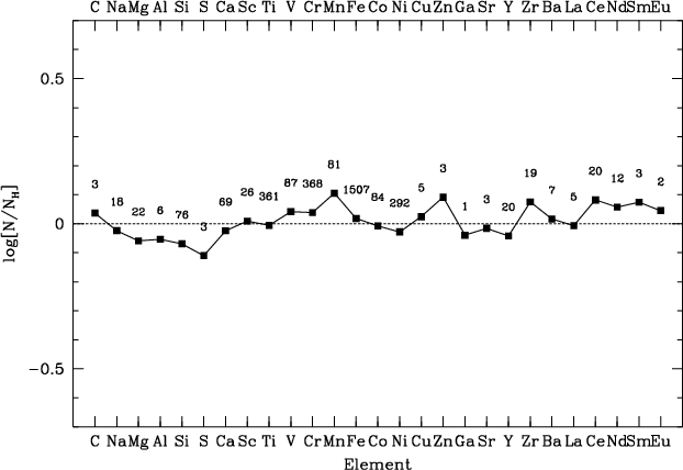	Figure 10: Same as Fig. 7, but with the difference for the Sun between this paper and Grevesse & Sauval (1998).
Open with DEXTER

In the solar case, the initial abundances were chosen different from the canonical one by some tenths of dex. The result of our analyzis is shown in Table 4 and in Fig. 10. A microturbulent velocity $\xi_{\rm micro}=0.79~{\rm km\,s^{-1}}$ was found, which is compatible with the value found by Blackwell et al. (1995, $\xi_{\rm micro}=0.775~{\rm km\,s^{-1}}$) when using the model from ATLAS9. Concerning the rotational velocities, it is important to note that the code does not implement macroturbulence treatment. Therefore, it is not possible to distinguish macroturbulent and rotational velocities. A value of $3.8~{\rm km\,s^{-1}}$ for the "rotational'' velocity was found. If we assume that the macroturbulence is isotropic, it is possible to get a more realistic value of the rotational velocity by doing a quadratic subtraction of the macroturbulent velocity. Takeda (1995b) found that the macroturbulence change from 2 to 4 $~{\rm km\,s^{-1}}$ depending of the choice of strong or weak lines. If we take a mean value of 3, we get $2.33~{\rm km\,s^{-1}}$ for the rotational velocity, which is slightly larger than the synodic value of $1.9~{\rm km\,s^{-1}}$.

The agreement for the abundances is always better than 0.1 dex except for S and Mn. The difference for S results from the value of $\log{\left[\frac{N({\rm el})}{N_{\rm H}}\right]}+12 = 7.33$ in Grevesse & Sauval (1998). However, both elements have photospheric abundances different from the meteoritic ones by as much as 0.1 dex. The meteoritic abundances are 7.20 and 5.53 for S and Mn respectively. Moreover, Rentzsch-Holm (1997) found an abundance of 7.21 for S, and in previous papers of Anders & Grevesse (1989), the S abundance is also 7.21, which is in perfect agreement with our value. Finally, the line list contains only 3 weak lines of about 15 mÅ, and therefore very sensitive to the continuum. Let us just stress that we do not maintain that our value is the correct one, but that for this element, the uncertainty is high. Concerning Mn, our value is close to the meteoritic value too. On the other hand, hyperfine splitting can have a significant impact and may lead to abundance overestimate of about 0.1 dex.

6 Conclusion

We have shown that our method of determining detailed abundances for A-F type stars works and that the ELODIE echelle spectrograph can be used to get accurate abundance determinations for Vega and the Sun. We achieve a high level of automation to extract spectra and analyze them. One line list covering the ELODIE spectral range was compiled and will be used for the following study of A-F stars. It includes new gf values for some critical lines determined using the solar spectrum.

The problem of the choice of stellar parameters which arose during the analysis of Vega is also a good justification to analyze a large sample of stars with one given method for determining stellar parameters ( $T_{\rm eff}, \log{g})$. The choice between a photometric or spectroscopic method is not so important since the uncertainty of these methods is comparable. Next it is important to determine abundances of all stars of the sample in a homogeneous way, and that will be possible with the method presented in this paper. This is our final goal for which automation will be crucial. Therefore, even if some uncertainties remain, the resulting errors will be systematic, and will not depend on the author's subjectivity.

Finally, our work is further justified by the commissioning of medium and high resolution multi-fibers spectrographs, because when an observer gets hundreds of spectra each night, he can no longer handle them by hand.

Acknowledgements

We thank Dr. G. M. Hill for providing the main program, and for his help in the early stages of development We thank Dr. Y. Chmielewski for useful and instructive discussions and for giving us some subroutines that proved very useful. We are grateful to Dr. R. O. Gray for his availability, his kindness and the pertinence of his answers to our numerous questions. Finally, the constructive comments of the referee, Dr. J. Landstreet, are gratefully acknowledged.

References

 
• Adelman, S. J., & Gulliver, A. J. 1990, ApJ, 348, 712 In the text NASA ADS  
• Anders, E., & Grevesse, N. 1989, Geochim. Cosmochim. Acta., 53, 197 In the text  
• Baranne, A., Queloz, D., Mayor, M., et al. 1996, A&AS, 119, 373 (BQ96) In the text NASA ADS  
• Barnard, A. J., Cooper, J., & Smith, E. W. 1974, J. Quant. Spec. Rad. Trans., 14, 1025  
• Barnard, A. J., Cooper, J., & Smith, E. W. 1975, J. Quant. Spec. Rad. Trans., 15, 429  
• Blackwell, D. E., Lynas-Gray, A. E., & Smith, G. 1995, A&A, 296, 217 In the text NASA ADS  
• Castelli, F., Gratton, R. G., & Kurucz, R. L. 1996, A&A, 318, 841 In the text NASA ADS  
• Chmielewski, Y. 2000, A&A, 353, 666 In the text NASA ADS  
• Cowley, C. R. 1996, in Model Atmospheres and Spectrum Synthesis, , ed. S. J. Adelman, F. Kupka, & W. W. Weiss, ASP Conf. Ser., 108, 170 In the text  
• Gigas, D. 1988, A&A, 192, 264 In the text NASA ADS  
• Gray, R. O., & Corbally, C. J. 1994, AJ, 107, 742 In the text NASA ADS  
• Grevesse, N., & Sauval, A. J. 1998, Space Sci. Rev., 85, 161 In the text  
• Hall, J. C., Fulton, E. E., Huenemoerder, D. P., Welty, A. D., & Neff, J. E. 1994, PASP, 106, 315 NASA ADS  
• Hill, G. M., & Landstreet, J. D. 1993, A&A, 276, 142 (HL93) In the text NASA ADS  
• Horne, K. 1986, PASP, 98, 609 In the text NASA ADS  
• Hubeny, I., Lanz, T., & Jeffery, C. S. 1994, TLUSTY and SYNSPEC: A User's Guide, Newsletter on Analysis of Astronomical Spectra, Univ. of St. Andrews In the text  
• Irwin, A. W. 1981, ApJS, 45, 621 In the text NASA ADS  
• Kupka, F., Piskunov, N. E., Ryabchikova, T. A., Stempels, H. C., & Weiss, W. W. 1999, A&AS, 138, 119 (VALD-2) In the text NASA ADS  
• Kurucz, R. L. 1979, ApJ, 40, 1 In the text  
• Kurucz, R. L. 1993, ATLAS9 Stellar Atmosphere Programs and 2 km s^-1 grid In the text  
• Kurucz, R. L. 1994, Kurucz CD-ROM 19, Solar Abundance Model Atmospheres for 0, 1, 2, 4, 8 km s^-1 
• Kurucz, R. L., Furenlid, I., Brault, J., & Testerman, L. 1984, The solar flux atlas from 296 to 1300 nm, National Solar Observatory Atlas No. 1, Sunspot, New Mexico In the text  
• Lemke, M. 1989, A&A, 225, 125 In the text NASA ADS  
• Lemke, M. 1990, A&A, 240, 331 In the text NASA ADS  
• Norlén, G. 1973, Phys. Scr., 8, 249 In the text  
• Palmer, B. A., & Engleman, R. Jr. 1983, Atlas of the Thorium Spectrum, Los Alamos National Laboratory, Los Alamos, New Mexico In the text  
• Press, W. H., Tukolsky, S. A., Vetterling, W. T., & Flannery, B. P. 1992, in Numerical Recipes, second edition (Cambridge University Press) In the text  
• Piskunov, N. E., Kupka, F., Ryabchikova, T. A., Weiss, W. W., & Jeffery, C. S. 1995, A&AS, 112, 525 (VALD-1) In the text NASA ADS  
• Qiu, H. M., Zhao, G., Chen, Y. Q., & Li, Z. W. 2001, ApJ, 548, 953 In the text NASA ADS  
• Rentzsch-Holm, I. 1997, A&A, 317, 178 In the text NASA ADS  
• Ryabchikova, T. A., Piskunov, N. E., Stempels, H. C., Kupka, F., & Weiss, W. W. 1999, Proc. of the 6th International Colloquium on Atomic Spectra and Oscillator Strengths, Victoria BC, Canada, Phys. Scr. T83, 162 (VALD-2) In the text  
• Sauval, A. J., & Tatum, J. B. 1984, ApJS, 56, 193 In the text NASA ADS  
• Takeda, Y. 1995a, PASJ, 47, 287 In the text NASA ADS  
• Takeda, Y. 1995b, PASJ, 47, 337 In the text NASA ADS  
• Tody, D. 1993, in IRAF in the Nineties, in Astronomical Data Analysis Software and Systems II, ed. R. J. Hanisch, R. J. V. Brissenden, & J. Barnes, ASP Conf. Ser., 52, 173 In the text  
• Valenti, J. A., & Piskunov, N. 1996, A&AS, 118, 595 In the text NASA ADS  
• Varenne, O., & Monier, R. 1999, A&A, 351, 247 In the text NASA ADS