J. H. J. de Bruijne¹ - A. P. Reynolds¹ - M. A. C. Perryman^1,2 - A. Peacock¹ - F. Favata¹ - N. Rando¹ - D. Martin¹ - P. Verhoeve¹ - N. Christlieb³

1 - Astrophysics Division, European Space Agency, ESTEC, Postbus 299, 2200AG Noordwijk, The Netherlands
2 - Sterrewacht Leiden, Postbus 9513, 2300RA Leiden, The Netherlands
3 - Hamburger Sternwarte, Gojenbergsweg 112, 21029 Hamburg, Germany

Abstract
We present observations of 11 quasars, selected in the range $z \approx 2.2$ -4.1, obtained with ESA's Superconducting Tunnel Junction (STJ) camera on the WHT. Using a single template QSO spectrum, we show that we can determine the redshifts of these objects to about 1%. A follow-up spectroscopic observation of one QSO for which our best-fit redshift (z = 2.976) differs significantly from the tentative literature value ( $z \approx 2.30$ ) confirms that the latter was incorrect.

Key words: instrumentation: detectors - galaxies: distances and redshifts - galaxies: high-redshift - quasars: absorption lines - quasars: emission lines - quasars: general

1 Introduction

Large ground and space telescopes combined with solid state detectors have revolutionized optical astronomy over the past two decades, yet deriving physical diagnostics of stars and galaxies still requires the somewhat indirect methods of filter photometry or dispersive spectroscopy to measure spectral features, energy distributions, and redshifts. The recent development of high-efficiency superconducting detectors (Perryman et al. 1993; Peacock et al. 1996) has introduced the possibility of measuring individual optical photon energies directly, and the first high time-resolution spectrally-resolved observations of rapidly variable sources such as cataclysmic variables and optical pulsars using these techniques have been reported (Perryman et al. 1999; Romani et al. 1999; Perryman et al. 2001; Bridge et al. 2001). Many extensive observational programmes which aim at determining the large-scale structure of the Universe, and galaxy formation and evolution (e.g., the Sloan Digital Sky Survey, Fan et al. 1999; the Anglo-Australian Telescope 2dF survey, Croom et al. 2001), demand high-efficiency extragalactic spectroscopy. Here we report the first optical measurements of spectral energy distributions of quasars using an imaging detector with intrinsic energy resolution, and show that we can determine their redshifts directly with excellent precision.

2 Observations

We observed 11 quasars in the redshift range z = 2.2-4.1, the sample comprising relatively bright high-redshift Lyman-limit quasars from the published literature (Sargent et al. 1989), supplemented by three lower redshift objects, two of which were discovered in objective prism-type surveys (Table 1). Observations used the ESA superconducting tunnel junction (STJ) camera, S-Cam2 (Rando et al. 2000), on the 4.2-m William Herschel Telescope, La Palma, between 2000 October 1-4. The camera is a $6 \times 6$ array of $25 \times 25$ $\mu$ m² ( $0.6 \times 0.6$ arcsec²) tantalum junctions, providing individual photon arrival time accuracies to about 5 $\mu$ s, a resolving power of ${\cal R} \approx 8$ at $\lambda = 500$ nm, and high sensitivity from 310 nm (the atmospheric cutoff) to about 720 nm (currently set by long-wavelength filters to reduce the thermal noise photons). All objects show strong Ly- $\alpha$ and CIV emission lines which, at these redshifts, will be present within our wavelength response range. Observations were made in modest seeing (1-1.5 arcsec at airmass X = 1), and at air-masses between X = 1.07-1.82.

Table 1: The 11 quasars observed. V gives the catalogue magnitude (probably questionable for 2143-158). T gives the exposure time in seconds, and $z_{\rm obs}$ our estimated redshift. The final two columns give the literature redshift and its source: S89 = Sargent et al. (1989) [spectroscopy]; M77 = MacAlpine et al. (1977) [objective prism]; C91 = Chaffee et al. (1991) [spectroscopy]; C85 = Crampton et al. (1985) [grens plate].
Obs. QSO V T $z_{\rm obs}$ $z_{\rm lit}$ Lit.

name (mag) (s) z

1 0000-263 17.5 600 4.095 4.111 S89

2 0052-009 18.2 1033 2.190 2.212 C91

3 0055-264 17.5 600 3.625 3.656 S89

4 0127+059 18.0 600 2.976 2.30 M77

5 0132-198 18.0 900 3.073 3.130 S89

6 0148-097 18.4 1800 2.845 2.848 S89

7 0153+045 18.8 600 2.978 2.991 S89

8 0302-003 18.4 900 3.263 3.286 S89

9 0642+449 18.5 900 3.366 3.406 S89

10 2143-158 21.2 1800 2.296 2.3 C85

11 2233+136 18.6 900 3.110 3.209 S89

**Table 1:** The 11 quasars observed. V gives the catalogue magnitude (probably questionable for 2143-158). T gives the exposure time in seconds, and $z_{\rm obs}$ our estimated redshift. The final two columns give the literature redshift and its source: S89 = Sargent et al. (1989) [spectroscopy]; M77 = MacAlpine et al. (1977) [objective prism]; C91 = Chaffee et al. (1991) [spectroscopy]; C85 = Crampton et al. (1985) [grens plate].
Obs.	QSO	V	T	$z_{\rm obs}$	$z_{\rm lit}$	Lit.
	name	(mag)	(s)			z
1	0000-263	17.5	600	4.095	4.111	S89
2	0052-009	18.2	1033	2.190	2.212	C91
3	0055-264	17.5	600	3.625	3.656	S89
4	0127+059	18.0	600	2.976	2.30	M77
5	0132-198	18.0	900	3.073	3.130	S89
6	0148-097	18.4	1800	2.845	2.848	S89
7	0153+045	18.8	600	2.978	2.991	S89
8	0302-003	18.4	900	3.263	3.286	S89
9	0642+449	18.5	900	3.366	3.406	S89
10	2143-158	21.2	1800	2.296	2.3	C85
11	2233+136	18.6	900	3.110	3.209	S89

3 Data reduction

Information on each detected photon consists of arrival time, x,ycoordinates of the junction, and an energy channel in the range 0-255. A photon of energy $E_{\rm p}$ (in eV) incident on a particular junction is assigned to an energy channel $E_i = G \cdot E_{\rm p} + C$ , where each pixel is characterised by its own gain G(in channels per eV) and offset C (in channels). Laboratory measurements have confirmed that all 36 junctions have a highly linear, albeit slightly pixel-dependent, energy response. Calibration consists of first bringing the observed energy channels to a common reference scale, corresponding to an arbitrary reference pixel, using a fixed gain map based on laboratory measurements. The offset of the reference pixel is constant (C = -2.0), and its gain is then the only free parameter in the absolute energy calibration. Small temporal gain variations resulting from bias voltage drifts and small detector temperature variations ( $\pm$ 0.01 K on the nominal operating temperature of $\approx$ 0.32 K) are monitored and calibrated.

Subtraction of the appropriate sky contribution for each quasar spectrum can in principle be based on the background signal in the outer array junctions, but given the small array size and seeing and refraction effects, we generally also took a nearby sky frame immediately following each quasar observation. Most observations were taken in astronomically dark time; QSO 2233+136, 2143-158, and 0148-097 were observed with the Moon setting, with background subtraction slightly less accurate.

4 Results

$\begin{figure}{\psfig{file=Dk021_f1.eps,width=7.02truecm,silent=,clip=} } \end{figure}$

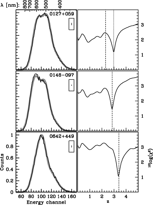Figure 1: Results for QSO 0127+059, 0148-097, and 0642+449. Left: the observed (black curves) and modeled (grey curves) energy channel distributions (arbitrary units). Insets indicate the estimated Poisson noise. Numbers above the top left panel show the mapping between energy channel and wavelength. Right: the corresponding dependence of $\chi ^2$ on z. Vertical dashed lines indicate the literature redshifts; the dotted line for QSO 0127+059 indicates the spectroscopic redshift reported in this letter (z = 3.04).

Open with DEXTER

We have determined each quasar redshift by comparing the calibrated energy distributions, $f_{\rm obs}(E_i)$ , with a single rest-frame composite quasar spectrum (Zheng et al. 1997) based on 284 Hubble Space Telescope Faint Object Spectrograph spectra of 101 quasars with z > 0.33. For a given gain G and redshift z, we construct the model energy-channel distribution $f_{\rm mod}(E_i)$ , as follows. The template spectrum is shifted from the rest frame to redshift z, and a mean accumulated absorption of the Lyman forest for this redshift is introduced (Møller & Jakobsen 1990) (all our objects are at high Galactic latitude, and we neglect Galactic reddening). The resulting spectrum is corrected for the mean atmospheric transmission at the relevant airmass, adjusted for the instrument and telescope efficiency curves and exposure time, transformed from wavelength spectra to energy-channel spectra, and finally convolved with a suitable Gaussian in order to account for the finite energy resolution of the detector. We then derive redshift z and gain G (and a normalization constant N), by minimizing the classical $\chi ^2$ function:

QSO 0127+059 is our single prominent outlier. It was discovered in a thin prism survey (MacAlpine et al. 1977), classified as a possible quasar, and tentatively assigned a redshift of $z \approx 2.30$ , but with an uncertain line identification. Although the quality of our fit is acceptable (Fig. 1), our derived redshift, z = 2.976, differs significantly from the literature value. We subsequently obtained a 1200 s spectrum of QSO 0127+059 (Fig. 3) with the Siding Spring Observatory 2.3-m telescope. The wavelength coverage (not optimised for quasar spectroscopy) was 345-537 and 560-753 nm, using the Double Beam Spectrograph with dichroic 1 and gratings 600B and 600R. We determine a spectroscopic redshift z = 3.04, which agrees with our estimate to about 2% (Fig. 2).

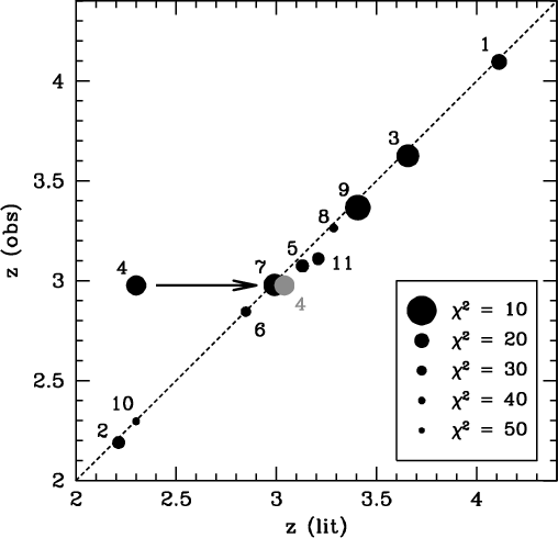$\begin{figure}{\psfig{file=Dk021_f2.eps,width=7.20truecm,silent=,clip=} } \end{figure}$	Figure 2: Observed versus literature redshifts. Numbers refer to the objects listed in Table 1, and symbol sizes correspond to $\chi ^2$ (smaller symbols indicating a poorer fit). QSO 0127+059 has an incorrect literature redshift of 2.30; our spectroscopic follow-up observation yields z = 3.04, moving the point to the position shown in grey. The dashed line shows the nominal 1:1 correlation.
Open with DEXTER

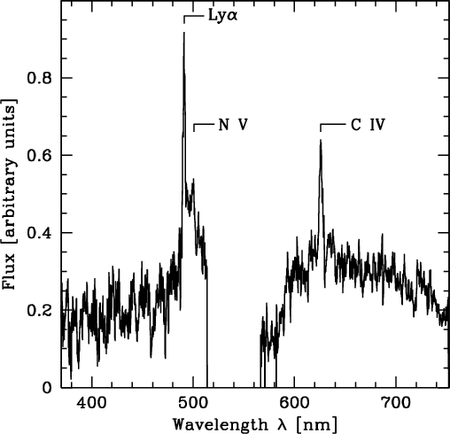$\begin{figure}{\psfig{file=Dk021_f3.eps,width=7.20truecm,silent=,clip=} } \end{figure}$	Figure 3: The spectrum of QSO 0127+059 obtained with the Siding Spring Observatory 2.3-m telescope, and smoothed with a 15 Å FWHM Gaussian. We determine z = 3.04; the resulting redshifted locations of Ly- $\alpha$ (121.6 nm), N `V` (124.0 nm), and C`IV` (154.9 nm) are indicated.
Open with DEXTER

A small systematic offset in the overall correlation, of $\approx$ 0.03 in z, can be attributed to a small mismatch in the shape of the energy broadening function or the overall throughput used in the modeling. The mean scatter for all observations is $\sigma_z = 0.03$ ; removing the systematic offset, 8 of the 11 objects agree to within 1%. Several factors, such as gain variations, erroneous sky subtraction or extinction correction (e.g., due to unmodeled seasonal Saharan dust in the atmosphere), or template mismatch at the object level (related to continuum slope, line ratios, etc.), may explain the observed spread. Formally, none of the fits is particularly good, in the sense that none of them has reduced $\chi^2 \approx 1$ . A key factor in $\chi ^2$ -statistics, however, is the absence of systematic errors, which will exist here in part due to template mismatch, although details are largely hidden as a result of the limited detector resolution. The general consistency between the models and the observations, and the pronounced, deep and narrow, minima in all $\chi ^2$ versus z plots, nonetheless indicate that our fits, as a set, are acceptable.

The pronounced minima are apparent in our data sets truncated a posteriori to observation times as small as, e.g. 10-20 s for the z = 4.1 object QSO 0000-263, where $\approx$ 350 source photons s^-1 were recorded.

5 Discussion

Although extraction of detailed physical information from the spectra is limited by the modest resolving power ( ${\cal R} \approx 8$ ) of the current device, a significant improvement in energy resolution can be expected in the future (Perryman et al. 1993; Peacock et al. 1997), and additional template spectra could then be used for model fitting. Our results show that low-resolution spectroscopy of faint extragalactic sources is possible with these devices, enabling the determination of redshift, and perhaps morphological type and emission and absorption line ratios (Jakobsen 1999; Mazin & Brunner 2000). Our instrument development is aimed at larger format arrays to facilitate sky subtraction and possibly for multi-object spectroscopy, and an increased energy resolution to improve physical diagnostic capability. An overall wavelength response extending further to the red, consistent with the fundamental device response characteristics, would also open up a larger accessible redshift range.

Direct determination of quasar redshifts

1 Introduction

2 Observations

3 Data reduction

4 Results

5 Discussion

References