with THEMIS spectropolarimetric mode MTR
(August 1998 campaign)
A&A 381, 227-240 (2002)
DOI: 10.1051/0004-6361:20011420
V. Bommier1 - J. Rayrole2
1 - Laboratoire "Atomes et Molécules en Astrophysique'', CNRS
UMR 8588 - DAMAp, Observatoire de Paris, Section de Meudon, 92195
Meudon, France
2 - Laboratoire "Physique du Soleil et de l'Héliosphère'', CNRS
UMR 8645 - DASOP, Observatoire de Paris, Section de Meudon, 92195
Meudon, France
Received 23 June 2000 / Accepted 28 November 2000
Abstract
The present paper is devoted to the search for the polarimetric
sensitivity level in observations of the Fe I 5576 Å line
performed with the THEMIS spectropolarimetric mode MTR on August 23
1998. This line is insensitive to the Zeeman effect and the present
work is thus useful to calibration purposes. The upper level of the
line is unpolarizable (J=0) and insensitive to the Hanle effect, and
the observations have been performed at disk center to avoid any
scattering polarization of lower level atomic polarization origin. In
the present paper, we describe the steps of a method that is the basis
of a data reduction code implemented on systems at the Meudon
Observatory for the interpretation of observations where a large
number (![]() 150) of images are averaged, and where the signal is in
addition averaged along the slit. First, we describe the numerical
methods used to determine the line position in the images, and to
perform operations on the profiles by FFT techniques (such as
translation, dilation, defocusing, apodization). Then, the
preprocessing steps are described: dark current subtraction,
destretching and flat-field correction. The polarization analysis is
then performed, based on the idea that, as the flat-field images are
unpolarized, they can be used to correct spurious polarization
occuring in the observations. As a result, the observed line is found
to be unpolarized, and a sensitivity of 2-4
150) of images are averaged, and where the signal is in
addition averaged along the slit. First, we describe the numerical
methods used to determine the line position in the images, and to
perform operations on the profiles by FFT techniques (such as
translation, dilation, defocusing, apodization). Then, the
preprocessing steps are described: dark current subtraction,
destretching and flat-field correction. The polarization analysis is
then performed, based on the idea that, as the flat-field images are
unpolarized, they can be used to correct spurious polarization
occuring in the observations. As a result, the observed line is found
to be unpolarized, and a sensitivity of 2-4
![]() is found
for the polarization degree in the neighboring continuum.
is found
for the polarization degree in the neighboring continuum.
Key words: methods: data analysis - methods: observational - techniques: polarimetric - techniques: spectroscopic - Sun: atmosphere - Sun: magnetic fields
The present paper reports results from observations obtained on August 23 1998, during the first observation campaign of the telescope THEMIS ("Télescope Héliographique pour l'Étude du Magnétisme et des Instabilités Solaires''), operating in its spectropolarimetric mode (MTR mode, "MulTi-Raies''). This mode aims to simultaneously record the spectrum in up to ten spectral ranges, in a given polarization state (i.e. polarization Stokes parameter). The polarization state can be changed for the following record, as well as the position of the slit on the disk. Thus, maps of solar regions can be recorded for a given polarization state. The interpretation of these polarized spectra can then lead to maps of the vector magnetic field because the four Stokes parameters can be recorded. By observing simultaneously different lines in the different spectral ranges, information on the depth behavior of the field vector can be retrieved. Moreover, the instrument has been designed in order to achieve high spatial accuracy. The major advantage of the THEMIS architecture is that it is a polarization-free telescope: the polarization analysis is performed before any oblique reflection, thus simplifying the calibration procedure.
The present observations and analysis are a preliminary step, in view of these general THEMIS objectives. Our aim is to determine the actual polarimetric sensitivity of THEMIS. To reach the highest polarimetric sensitivity, we have ignored the spatial resolution, and averaged the data along the slit, as well as recorded 300 images for each observation, and averaged on the best number of them. Such an observing procedure is also a preliminary step for further observations in quiet sun regions, whose scientific objectives are described in more details in Sect. 2.1. They have been performed in the Fe I 5576 Å, a line that is insensitive to atomic polarization in the upper level because it is a J=0 level, as well as to the Zeeman effect. Moreover, the observations have been performed at disk center, in a quiet region, so that neither magnetic field nor scattering polarization effects are expected.
The observations and polarimetry techniques are described in Sect. 2. The numerical methods used for the data processing are described in Sect. 3. The data analysis is described in Sect. 4, and the results are finally discussed in Sect. 5 in terms of polarimetric sensitivity of THEMIS in these particular observations.
The present paper is the description of a method that is at the basis of a data reduction code that is implemented on the Meudon Observatory computer systems. The flow-chart of the reduction procedure and code is given in Appendix A.
Among the different polarimetric observations that can be performed on the
Sun, there are some that require an especially high value of sensitivity.
These are: those aimed at atomic polarization detection, such as quiet sun
center-to-limb variation of the scattering polarization, eventually modified
by the Hanle effect. In such observations, the spatial resolution can be
degraded by averaging along the slit, in order to increase the polarimetric
sensitivity. Atomic and scattering polarizations are weak: typically, less
than 1%. As every component of the THEMIS telescope has been designed
to achieve an absolute polarimetric accuracy of ![]() 10-3 without
any correction, it is necessary to increase the sensitivity by averaging
pixels, in order to obtain sufficient sensitivity to measure the signal
expected in such observations. That is why the present observations have
been averaged along the slit and over a large number of images.
10-3 without
any correction, it is necessary to increase the sensitivity by averaging
pixels, in order to obtain sufficient sensitivity to measure the signal
expected in such observations. That is why the present observations have
been averaged along the slit and over a large number of images.
The polarization analyzer, which is installed at the F1 focus of the Ritchey-Chrétien telescope, is composed of two achromatic quarter-wave plates and a polarizing beam splitter. At the output of the polarimeter, the two polarized beams, whose intensity are respectively (I+S) and (I-S), (where S is one of the 3 Stokes parameters (Q,U,V), or a combination of them, depending on the quarter-wave plates orientation), follow different paths ("transfer optics'', F2) after having passed through two different slits, enter separately the spectrograph and are recorded on two different cameras at the exit of the spectrograph. Thus, a given Stokes parameter can be retrieved by subtracting images taken at the same time on two different cameras and after the beams have followed different optical paths that, obviously, cannot be strictly identical. A method is proposed in the present analysis to evaluate and take into account such differences. This method is based on the idea that, assuming that the flat-field images are unpolarized, they can be used to correct the observations for the polarization signals spuriously induced by the differences in the cameras and in the ray path.
The sequence of flat-field images has been taken on the Sun itself, in order
to have intensities as similar as possible in the flat-field and in the
observations. Since defocusing the telescope is not desirable, the
flat-field images have been taken by rapidly moving the solar disk on the
entrance slit, along an ellipse with randomly variable axes (in length as
well as in direction). To obtain unpolarized flat-field images, the elliptic
motion is performed outside any active feature. The random character of the
procedure ensures that no regularity will bias the data, and that the slit
will not pass twice on the same solar point. About 300 images have been
recorded for each position of the polarization analyser, corresponding to
![]()
![]() and
and ![]() .
.
The line observed was Fe I 5576 Å, which is insensitive to the
Zeeman effect. The upper level of the line is unpolarizable (J=0), which
implies that this line cannot display scattering polarization, or the Hanle
effect (discarding eventual lower level polarization effects, as those
suggested by Trujillo Bueno & Landi Degl'Innocenti 1997; Landi Degl'Innocenti 1998). As the aim of the present
observations was to detect the polarimetric sensitivity of the instrument
while avoiding any magnetic field or scattering polarization effects, the
observations were performed at disk center, with a slight movement of the
slit around it, in order to average on eventual spatial structures. This
movement was performed by using the same facility as for the flat-field, but
with much smaller lengths of the ellipse axes. Again, about 300 images were
recorded for each position of the polarization analyzer, corresponding to ![]()
![]() and
and ![]() .
The integration time was 400 ms per image.
An example of the raw data is given in Fig. 1.
.
The integration time was 400 ms per image.
An example of the raw data is given in Fig. 1.
The magnifying factor of the optics was such that the dispersion was 14.1 mÅ per pixel of the cameras.
![\begin{figure}
\par\includegraphics[width=15.8cm,clip]{aa1910F1.eps}
\end{figure}](/articles/aa/full/2002/01/aa1910/img7.gif) |
Figure 1: Raw images of the Fe I 5576 Å line profile observed at disk center, obtained with THEMIS on 1998 August 23, in the two channels I+Q and I-Q. The horizontal dimension of the images is the dispersion, and the vertical dimension is the spatial dimension along the slit. |
| Open with DEXTER | |
As it can be seen in the raw data in Fig. 1, the line is not perpendicular to the dispersion direction (the horizontal axis), and it is necessary to determine as precisely as possible the line position along each pixel row, and then to translate the pixel row in order to perform the line destretching. Our flat-field technique also requires destretching (see the next section). We present in this section the numerical methods that we used to determine the line position along a pixel row, and to translate it with a non-integer step, and eventually to dilate or contract it. These two last methods make use of FFT ("Fast Fourier Transform''). Another FFT method is also proposed to "defocus'' (i.e. broaden without displacing) a line profile, if necessary. Finally, an apodization technique for FFT based on cubic spline interpolation is described. The data analysis is performed by using the IDL software, which contains a number of internal functions. In the following, we describe the different steps of the methods, that make use of the internal functions that can be also found in other softwares.
As all the steps of the data analysis, present or future, require only the
determination of a relative displacement as precisely as possible, we
have used the method developed by Rayrole (1967), in which
the parameter that we determine is not the line minimum (whose precise
determination in discrete data may be difficult), nor the line center of
gravity, but the line bisector position at a given depth in the profile
(this depth being determined by the parameter ![]() introduced below). We
describe this method below. The only requirement of our analysis is that the
line parameter that is determined is always the same, in order to retrieve
the relative displacements in the subsequent analysis.
introduced below). We
describe this method below. The only requirement of our analysis is that the
line parameter that is determined is always the same, in order to retrieve
the relative displacements in the subsequent analysis.
A profile is given, for instance, by a row of pixels of the image. In order
to reduce the noise in the data that could disturb the subsequent analysis,
the first step is to perform a convolution of this vector of data with a
normalized stepwise function of width ![]() pixels
pixels
 |
(1) |
The second step is to perform the differences between the convolved function
values p(i) taken at pixels separated by a quantity
![]() that will be
called the "slit gap'' (as if two theoretical slits were placed at positions i and
that will be
called the "slit gap'' (as if two theoretical slits were placed at positions i and
![]() ). We compute
). We compute
 |
(2) |
This method is very sensitive, robust and precise. For typical values such
as those of our observations (see the number of pixels inside the line
profile in Fig. 7: ![]() 20 pixels in twice the line
width), we have chosen
20 pixels in twice the line
width), we have chosen
| (3) |
Tests performed on randomly noised theoretical profiles with a similar pixel sampling have shown that the accuracy of this line position determination is a few hundredths of a pixel.
To increase the precision of the method, it is possible to perform iterations: after the line position is determined by the bisector method, the entire row is then translated (using the FFT method described in the following Sect. 3.2.1) to put the line position on an integer pixel number; the line position is again determined by the bisector method, and found slightly different, due to the effect of the linear interpolation; the corresponding translation towards an integer pixel number is performed, and so on. The convergence (position variation smaller than 10-4 pixel) is typically reached in 3 iterations.
To destretch, it is necessary to translate each pixel row with a fractional step along the dispersion dimension. To correct for the magnifying difference between the channels, it is necessary to slightly dilate the profile obtained in one of the two channels. For these two purposes, we have settled on methods that modify the phase factor that enters the FFT ("Fast Fourier Transform'') of the line profile. These methods are in common use. This principle was suggested by Keller (1999). However, when completed by the apodization technique described in Sect. 3.2.4, we have found this combination powerful, such that we describe below the entire method.
If the profile is given by the function f(x), where x is a pixel number,
the discrete Fourier transform F(u) of the f(x) function is given by
If a translation of the profile of the quantity ![]() towards the right
hand side is to be done, the new abscissae
towards the right
hand side is to be done, the new abscissae
![]() are related to the
old ones x by
are related to the
old ones x by
 |
(6) |
| = | ![$\displaystyle \sum\limits_{u=u_{\min }}^{u_{\max }}\left[ F(u)\;\exp
[-2{\rm i}\pi u\Delta x/N]\right] \;$](/articles/aa/full/2002/01/aa1910/img27.gif) |
||
| (7) |
![\begin{figure}
\par\includegraphics[width=7.9cm,clip]{aa1910f2.eps}
\end{figure}](/articles/aa/full/2002/01/aa1910/img30.gif) |
Figure 2: Example of FFT line minimum determination. The Sr I 460.7 nm line profile, extracted from one of our limb observations of 1999 September 22, has been dilated 10000 times by applying the FFT dilation method described in the text. The figure shows the center of the dilated profile, and the dot-dashed line indicates the minimum position. The small stairs around the minimum are due to the numerical accuracy of the computation, which has been performed in double precision. The minimum position is in fact the middle of the lowest stair. The absissæ are pixels of the dilated profile: due to the dilation, each pixel step of the figure is 0.0001 pixel steps of the initial profile. |
| Open with DEXTER | |
For a linear dilation (contraction) of the profile, one has
 |
(8) |
![\begin{displaymath}f_{{\rm D}}(x)=\sum\limits_{u=u_{\min }}^{u_{\max }}F(u)\;\exp [2{\rm
i}\pi ux/(gN)].
\end{displaymath}](/articles/aa/full/2002/01/aa1910/img34.gif) |
(9) |
This method can be used for any value of g, near unity as well as very large. Values near unity are used for correcting the data for differences in the magnifying factor between the two channels. We also used this method to build a precise line position determination method, that we applied to our THEMIS 1999 data (see an example in Fig. 2), by applying very large g factors to the observed line profiles, in order to detect the line minimum with a high fractional pixel accuracy. Tests have shown that the accuracy of this Fourier interpolation seems to be limited by numerical accuracy only: using double precision calculations (as it is necessary for good FFT calculations), one can introduce up to 105points in twice the halfwidth of a line profile, with reasonable results (for higher values, regular stairs appear in the profile that are of numerical origin. Such stairs are slightly visible in Fig. 2). In our 1999 data, where we treated profiles having about 15 points in 4 times the halfwidth, we applied g=104 to detect the line minimum (see Fig. 2), with the corresponding accuracy of 0.0001 pixel (this is a numerical accuracy that does not take into account possible noise in the data). The dilation is applied after having extracted the full profile by selecting two continuum points, one on the adjacent left side and one on the adjacent right side of the line of interest. It can be seen in the example given in Fig. 2 that such a Fourier interpolated line profile is of very high quality and is very symmetrical, and that the line center is well determined by this method. However, this was not always the case in all the lines that we have thus treated, probably when the ADU level in the line center is too low.
This method can also be denoted as "Fourier interpolation''.
![\begin{figure}
\par\includegraphics[width=7.9cm,clip]{aa1910f3.eps}
\end{figure}](/articles/aa/full/2002/01/aa1910/img35.gif) |
Figure 3: Application of the defocusing method described in Sect. 3.2.3. The sharpest line is the Sr I 5607 Å as observed during the 1999 campaign, and the broadest line is the result of the application of our defocusing method to this line. |
| Open with DEXTER | |
Though it has not been used with the THEMIS 1998 data, but with the 1999 data that will be presented in a further paper, we have built a FFT method able to provide line "defocusing'', i.e. this method is able to increase the width of a line given on a number of individual pixels. The line depth is modified also, but in such a manner that the line integral (the equivalent width) is not modified, by using the normalization conditions as given below. The line position is unchanged. An example of its application is given in Fig. 3, where the sharpest line is the Sr I 5607 Å observed during the 1999 campaign, and the broadest line is the result of the application of our defocusing method to this line.
In our 1999 data, important focusing differences between the two channels occur, resulting in a difference of 3% in line width between the two channels, that prevents further polarization analysis. Practically, one of the two cameras was probably out of focus. The result is a broadened line in this channel that results from the convolution of the line with an instrumental profile. Deconvolving is a very complex operation, requiring much information. As a first step, we successfully tried another method: broadening the sharpest (well focused) line of the two channels, in order to get the same line width between the two channels. This approach is justified by the fact that the expected signal (the scattering polarization) does not change significantly along the line profile.
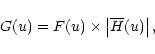
The objective of the method is then to convolve the line f(x) with a given function h(x). As we are looking for a small broadening (3% in the above example), the convolving function h(x) will be sharp, and consequently not well defined on a small number of pixels. On the contrary, in the Fourier (frequency) space, the Fourier transform H(u) of h(x) will be broad and well defined on a large number of pixels. The idea is then to perform the convolution in Fourier (frequency) space, where the convolution is transformed in a usual simple product.
The main idea of our method is to use as a broadening function h(x), a function extracted from the line to be broadened itself, in order to introduce no other information in the treatment other than that contained in the data themselves. Thus, no additional information enters our defocusing process: only the line to be broadened and the FFT are used. We present this method below.
A portion h0(x) of the spectrum is extracted by selecting two continuum
points, one on the adjacent left side and one on the adjacent right side of
the line of interest. h0(x) then contains the line profile only, in
absorption. The first step is to subtract the continuum and change the line
sign in order to get a single emission profile h(x) without any continuum
 |
(11) |
 |
(12) |
The broadened Fourier transform
![]() of
of
![]() is
then computed, using a broadening technique analogous to the one described
above for the dilation/contraction, but now applied to frequencies, with
is
then computed, using a broadening technique analogous to the one described
above for the dilation/contraction, but now applied to frequencies, with
 |
(13) |
The Fourier transform F(u) of the total spectrum f(x) is computed
following Eq. (4) and using the internal FFT routine, and the
convolution is performed in the Fourier (frequency) space, by multipying
F(u) by the modulus of
![]()
Due to the fact that it is based on a convolution, this method is only able
to broaden a profile: no profile sharpening is possible with such a method,
though, in principle, it would be possible to replace the multiplication in
Eq. (15) by a division. We have, however, tried to sharpen
profiles, and found that such a sharpening method works only for small
values of the q factor, when
![]() is not too small even at
high frequencies.
is not too small even at
high frequencies.
We have applied this method to our 1999 data, where a 3% difference in line width between the two channels occured. We found a q factor able to reasonably adjust the two profiles, but further problems (probably scattered light) prevented us from realizing the polarization analysis. We finally treated these data by applying beam exchange techniques that will be described in a forthcoming paper, that perform an average between the two different line widths; thus, when beam exchange techniques are used, it is not necessary to correct the data for such a difference (when it is small).
It is important to point out that the results of the two methods described above on dilation/contraction, on the one hand, and defocusing, on the other hand, are different: in the dilation/contraction method, the minimum intensity of the line (for an absorption line - both methods could obviously apply to emission lines: only Eq. (10) should be ignored in this case) is unchanged, but the line is broadened and displaced, and this method is just an interpolation between pixels. In the defocusing method, the line width and intensity are both modified, but the line position and equivalent width are unchanged.
The use of FFT methods generally requires apodization of the function f(x), before applying the method. If the two extreme values f(1) and f(N)are different, parasitic oscillations appear when a direct followed by an inverse FFT is performed: this phenomenon is corrected by "apodizing'' f(x).
In our work on the THEMIS 1998 data, this has been avoided, because the black borders at the right and left sides of our images (see Fig. 1), ensure "natural apodization'', with values of the same order of magnitude at the two edges of our pixel rows. However, further requirements arising during the treatment of the 1999 data (which will be published in a further paper) have led us to build an apodization method based on cubic spline interpolation that we present below.
As the internal FFT routines run much faster when N is a power of 2, the idea is to extent the given length of the vector to the next upper power of 2 before performing the FFT operations: in the THEMIS data, our vectors have 382 elements (the width of the THEMIS CCD cameras) that we extend to 512 elements. The FFT computations are performed with the 512-elements vector, and the added part of the vector is removed at the end of the calculation.
The apodization is ensured if the added part of the vector is such that continuity of the new vector and of its first derivatives are ensured when the left extremity is joined to the right extremity (when a periodic function would be constructed with the new vector by using, as the period, the new vector length). Our idea has been to use cubic spline interpolation, using the 3 first and 3 last points of the initial vector, to determine the content of the part added for constructing the new vector.
In our THEMIS 1998 data treatment, where we did not make apodization, we have completed the 382-elements vectors (containing the line profiles) to 512-elements vectors by adding 0 values (due to the black borders at the left and right sides of the images, the values at the edges of the 382-elements vector are around zero after dark current subtraction). For our correction vector (see next section), whose values lie around unity, we have completed the vector by adding 1 values.
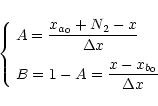
In our apodization method based on cubic spline interpolation, we denote as
a0, a1 and a2 (from left to right) the 3 first points of the
initial vector (left extremity), with abscissæ (pixel values)
xa0<xa1<xa2, and values (content of the vector) that we
denote as ya0, ya1 and ya2. Similarly, we denote as
b2, b1 and b0 (from left to right), the 3 last points of the
initial vector (right extremity), with abscissæ (pixel values)
xb2<xb1<xb0, and values (content of the vector) that we
denote as yb2, yb1 and yb0. The left and right
extremity abscissæ are then xa0 and xb0. We assume that
the abscissæ are pixel numbers, such that
 |
(16) |
| N=xb0-xa0+1 | (17) |
![\begin{displaymath}N_{2}-N\geq \max [20,0.2\times N]
\end{displaymath}](/articles/aa/full/2002/01/aa1910/img47.gif) |
(18) |
 |
(19) |
| (20) |
We denote as
![]() and
and
![]() the second derivatives in a1 and b1
the second derivatives in a1 and b1
 |
(21) |
| = | ![$\displaystyle \frac{2+3\Delta x}{6}\left[
\frac{y_{a_{0}}-y_{b_{0}}}{\Delta x}\right]$](/articles/aa/full/2002/01/aa1910/img56.gif) |
||
![$\displaystyle -\frac{1+\Delta x}{3}\left[ (y_{b_{0}}-y_{b_{1}})+\frac{1}{6}
y_{b_{1}}^{\prime \prime }\right]$](/articles/aa/full/2002/01/aa1910/img57.gif) |
(22) | ||
![$\displaystyle +\frac{\Delta x}{6}\left[ (y_{a_{0}}-y_{a_{1}})+\frac{1}{6}
y_{a_{1}}^{\prime \prime }\right],$](/articles/aa/full/2002/01/aa1910/img58.gif) |
| = | ![$\displaystyle -\frac{2+3\Delta x}{6}\left[
\frac{y_{a_{0}}-y_{b_{0}}}{\Delta x}\right]$](/articles/aa/full/2002/01/aa1910/img60.gif) |
||
![$\displaystyle -\frac{1+\Delta x}{3}\left[ (y_{a_{0}}-y_{a_{1}})+\frac{1}{6}
y_{a_{1}}^{\prime \prime }\right]$](/articles/aa/full/2002/01/aa1910/img61.gif) |
(23) | ||
![$\displaystyle +\frac{\Delta x}{6}\left[ (y_{b_{0}}-y_{b_{1}})+\frac{1}{6}
y_{b_{1}}^{\prime \prime }\right],$](/articles/aa/full/2002/01/aa1910/img62.gif) |
![\begin{displaymath}\Delta =\frac{1}{9}\left[ 1+\frac{\Delta x}{2}\right] \left[ 1+\frac{3\Delta
x}{2}\right]
\end{displaymath}](/articles/aa/full/2002/01/aa1910/img63.gif) |
(24) |
Then, for a given pixel x located in the added part of the vector
(
xb0<x<xa0+N2), the y value (content of the vector) is
given by
 |
(25) |
 |
(26) |
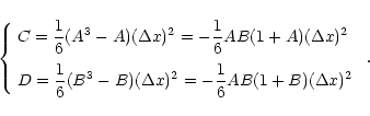 |
(27) |
Notice, however, that in our defocusing technique (Sect. 3.2.3), apodization has to be applied to the initial total spectrum f(x), but not to the h(x) convolving function, which has to be completed by 0 values.
![\begin{figure}
\par\includegraphics[width=14.4cm,clip]{aa1910F4.eps}
\end{figure}](/articles/aa/full/2002/01/aa1910/img68.gif) |
Figure 4: Preprocessed images (above) and flat-field matrix images (below) of the Fe I 5576 Å line profile, obtained with THEMIS on August 23 1998, in the two channels I+Q and I-Q. The preprocessing step includes dark current correction, destretching and flat-field correction, using the respective flat field matrices displayed in the lower part of the figure. For the derivation of the flat-field matrices, see text. |
| Open with DEXTER | |
We have found these FFT methods extremely powerful: very high quality interpolations are obtained, and rapid calculations are done when the internal routines can be used. No additional information apart from that contained in the data is introduced to achieve the interpolation. The origin of this power lies probably in the fact that the FFT is a development over an ensemble of functions that form a basis of the subspace of functions that do not contain frequencies higher than the Nyquist frequency, which results in the property that no information is lost when the function is reconstructed in the inverse FFT. Obviously, the details of the initial function that correspond to frequencies higher than the Nyquist fequency are definitely lost.
The data processing is composed of two main steps: preprocessing (dark current correction, destretching, flat-field correction), that is performed independently in each of the two polarization channels, and polarization analysis processing, in which the subtraction of the two channels is performed.
The flow-chart of our data processing method and code is given in Fig. A.1.
For the dark current, flat-field and observations images, 150 raw images are averaged.
The dark current average image is subtracted from the data average image (flat-field and observation).
It has been observed on the black borders (right and left) of the images that the average value of the dark current shows important slow variations. We therefore performed a correction to the dark current image subtraction: we averaged the values along each pixel row, in the two left and right dark borders of the raw images, and evaluated the average on the same pixels of the dark current image. We added to the dark current image subtraction a correction given by the difference between these two average values, which takes into account the average slow variation of the dark current. The fluctuations of the dark current are not taken into account; they may be responsible for the final noise in the results.
These slow variations were very important in the THEMIS first
observations: when this last correction was not performed, parasitic
polarization of up to ![]() was obtained for the observations.
was obtained for the observations.
The position of the line profile on the flat-field image is determined using the method described in Sect. 3.1, along each pixel row. When plotted as a function of the row number, this position shows a (noised) inclined and curved behavior, that has to be fitted with a second-order polynomial. Performing second order polynomial interpolation of the line positions leads to 3 coefficients defining the fit curve. Each pixel row is then translated by the difference between the fitted second order curve and a given position, in order to align all the rows to this position, using the second order fit. As a result, the line profile becomes aligned, with noise, along a column.
In practice, we perform the coefficient determination in two steps: we first perform a raw destretching, assuming a linear inclination of the line between two mouse-acquired values. The aim of this preliminary step is to determine a rather sharp "working window'' around the line, in which the line position determination method can be applied without being biased by possible neighboring lines. We then perform the second order polynomial fit of the line positions, and get the fit coefficients. However, we perform the final destretching of the raw image in only one step, by combining the mouse-acquired and fitted coefficients.
The determination of the coefficients is performed on the flat-field images
(after dark current correction). These coefficients are applied to both the
flat-field and observation images, both being corrected for the dark current.
![\begin{figure}
\par\includegraphics[width=7.9cm,clip]{aa1910f5.eps}
\end{figure}](/articles/aa/full/2002/01/aa1910/img70.gif) |
Figure 5: The upper part of the figure displays the two profiles averaged along the slit, obtained from the flat-field images. Full line: channel I+Q. Dotted line: channel I-Q; the average value of the intensity in this channel has been scaled to the average value of the intensity in the other channel. The lower part of the figure displays the polarisation (difference divided by sum) of the two profiles plotted in the upper part. The vector of correction used in the following data processing is the ratio between these two profiles. |
| Open with DEXTER | |
The average profile is determined by averaging the destretched flat-field image along each column, between two limits, to eliminate the black borders that are present at the top and bottom of the images.
The flat-field matrix is then obtained by dividing each row of the destretched flat-field image by this average profile (the left and right black borders are also excluded from the matrix).
Examples of flat-field matrices are given in Fig. 4. It can be seen that in one of the two channels, two embedded systems of fringes are retrieved in the flat-field matrix. These fringes are indeed present in the raw images, as a close inspection of Fig. 1 shows. They will then be corrected by applying the flat-field correction.
The destretched observation image is then divided by the flat-field matrix, in their common area, after eliminating the dark borders in the top, bottom, right and left of the images.
It can be seen in Fig. 4 (top panel) that the horizontal dark lines that are present in the raw data (see Fig. 1), and that are due to scratches on some optical pieces, or to dusts in the slit, are not completely removed by the flat-field correction. This is due to the fact that the image moves slightly on the camera over time (movement induced during the field derotation, needed due to the alt-azimuthal mount), so that these dark lines do not have exactly the same position in the flat-field and observation images, which are not taken at the same time.
![\begin{figure}
\par\includegraphics[width=7.9cm,clip]{aa1910F6.eps}
\end{figure}](/articles/aa/full/2002/01/aa1910/img71.gif) |
Figure 6: Upper part: polarisation profile Q/I obtained from the disk center images, after preprocessing and application of the correction vector (see text and Fig. 5). Q and I have been separately averaged along the slit. As in Fig. 5, the average value of the intensity in the I-Q channel has been scaled to the average value of the intensity in the I+Q channel. Lower part: modulus of the FFT of the Q/I signal, showing peaks corresponding to fringes remaining after the flat-field correction. These fringes are further eliminated by applying sharp band-stop filters centered on each of the peaks (see text). |
| Open with DEXTER | |
At this stage, it has to be stressed that the flat-field technique applied in the present work is not "isotropic'' in the image: well localized faults (such as dust) and horizontal faults are retrieved in the flat-field matrix, and are then corrected when this matrix is applied. However, the vertical (i.e. parallel to the line) features are eliminated from the flat-field matrix by the present technique, because this technique is founded on the idea that the line itself is not to appear in the flat-field matrix. Thus, vertical fringes would not be corrected by such a technique. As seen in Fig. 5 (upper panel), the continuum in the average profile shows an inclined behavior that corresponds to a vertical inclination in the image (i.e. the same inclination along each pixel row), that consequently cannot be corrected by our flat-field procedure. The precise origin of this inclination is unclear for the moment. Moreover, it may be seen in Fig. 5 that this inclination is not the same in the two polarization states to be subtracted. The origin of this difference is also unclear for the moment, and may be different from the origin of the inclination itself. This inclination difference, that also cannot be corrected by our flat-field technique, is one of the features that is taken into account in the correction vector that we further introduce in the analysis (see Sect. 4.2.3).
As seen in the lower panel of Fig. 4, the Fe I 5576 Å line is slightly visible in the flat-field matrix, contrary to what is theoretically expected. This is probably due to the fact that, in the present observations, the excursion of the slit on the solar disk during the flat-field recording is a non-small fraction of the solar radius: thus, due to the solar rotation and Doppler effect, the spectral position of the Fe I 5576 Å line varies from record to record of the flat-field images. Because 150 images are averaged in order to get the flat-field matrix, this results in a net broadening of the line and of the derived average profile. During the following 1999 campaign, the excursion was chosen smaller, and the line is therefore even less visible in the flat-field matrix.
![\begin{figure}
\par\includegraphics[width=16cm,clip]{aa1910F7.eps}
\end{figure}](/articles/aa/full/2002/01/aa1910/img72.gif) |
Figure 7: Stokes profiles (averaged along the slit) of the Fe I 5576 Å line observed at disk center, after data processing and remaining fringe elimination (see Fig. 6). |
| Open with DEXTER | |
All the preprocessing steps being performed on the images obtained in each of the two channels, the objective of the processing step is to perform the image subtraction in order to derive the polarization. A vector of correction is evaluated from the flat-field average profiles, and then applied to the observation data to correct them for the spurious polarization (it is assumed that the flat field images are unpolarized).
As already stated, the analysis is performed on the average of 150 raw images, though, in principle, the same analysis might be performed on the individual images.
The images are averaged along columns (i.e. along the slit), and the subtraction is performed on the average profiles of the two images corresponding to a given Stokes parameter.
A slight difference between the two channels can be found in the magnifying factor resulting from the camera optics. In the present analysis, where we work on slit-averaged data, we determine the magnifying difference along the dispersion axis by evaluating the positions of two lines (one of them very weak), respectively on the right and left sides of the Fe I 5576 Å line, on the two average profiles of the flat-field images. One of the two profiles is corrected for this magnifying difference by applying the FFT method described in Sect. 3.2. The magnifying factor to be applied to this profile is found to be of the order of g=1.01. This magnifying factor, retrieved from the flat-field images, is applied to the flat-field and observation average profiles.
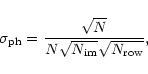
At this stage, it is possible to evaluate the photometric noise in the data
by applying all the preceding treatment to the individual observation
images, and by selecting a point on continuum. The standard deviation of the
intensity recorded at this wavelength is evaluated for N images and then
divided by ![]() .
This operation is repeated from N=2 to the total
number of images, which is about 300 in our data. We have thus obtained the
lowest value at the level
.
This operation is repeated from N=2 to the total
number of images, which is about 300 in our data. We have thus obtained the
lowest value at the level
![]() of the continuum intensity,
for N=150. For increasing values of N>150, this photometric noise level
increases, indicating that 150 is the best number of images to be averaged.
In all the present analysis, we have then used averages of 150 images.
of the continuum intensity,
for N=150. For increasing values of N>150, this photometric noise level
increases, indicating that 150 is the best number of images to be averaged.
In all the present analysis, we have then used averages of 150 images.
![\begin{figure}
\par\includegraphics[width=16cm,clip]{aa1910F8.eps}
\end{figure}](/articles/aa/full/2002/01/aa1910/img75.gif) |
Figure 8: Dotted line: same as Fig. 6. Full line and crosses: noise filtered profiles obtained by thresholding the wavelet transform of the Q signal (Daubechies-20 wavelets have been used). |
| Open with DEXTER | |
The birefringence in the entrance window (in which temperature differences
up to
![]() C can be detected, leading to non-axisymmetrical
stress), the scattered and stray light, and any difference between the two
optical paths, all may be responsible for parasitic polarization in the
analysis. We propose to determine globally this parasitic polarization by
assuming that the flat-field images are unpolarized, and then to correct the
observations for the channel difference thus retrieved.
C can be detected, leading to non-axisymmetrical
stress), the scattered and stray light, and any difference between the two
optical paths, all may be responsible for parasitic polarization in the
analysis. We propose to determine globally this parasitic polarization by
assuming that the flat-field images are unpolarized, and then to correct the
observations for the channel difference thus retrieved.
The first step is to translate the two average profiles of the flat-field images towards the same position. To do this, the FFT method described in Sect. 3.2 is used.
Due to the different polarization states in the two channels at the output of the polarimeter, this polarization combines with the reflections inside the spectrograph, and, as a result, the intensity levels in the two channels are widely different. The second step is to adjust the continuum of the two profiles to the same level. Because in our data the continua appear to be non-linear, we multiply one profile by the ratio of the average values of the two profiles, restricted to their overlapping part. Though such a method would not be convenient for a highly sensitive polarization analysis, it is sufficient for the present analysis where the polarization accuracy remains above 10-4. We call this method the "mean value'' method. Alternatively, it would be possible to choose two points well situated in the continuum and, assuming a linear behavior of the continuum between these two points, to adjust the two continua. We have also tried this procedure, and found no important difference in the final result of our analysis.
After having thus adjusted the intensities of the two average profiles of the flat-field images, we perform the ratio of these two profiles, obtaining thus a vector of values around 1, to be applied to the observation profiles, and that we call the "correction vector''. In Fig. 5, we have plotted the two adjusted continua (by our "mean value'' method), and the polarization that would result from the subtraction of these two flat-field profiles. It may be seen in the figure that this polarization (channel difference) is of the order of 1-2%, at 5576 Å. This polarization is the content of the correction vector.
For applying this correction vector to the observation profiles, we have first to translate the two observation profiles towards the same position as the one previously chosen for the flat-field profiles (by applying the FFT method described in Sect. 3.2), and to select the overlapping part among all the flat-field and observation profiles. The observation profile in the second channel is then multiplied by the correction vector. The observation profiles are then corrected for the intensity difference by applying our "mean value'' method (the ratio of mean values is different from the one of the flat-field images), and the resulting observed polarization is then evaluated, by performing the difference of the two profiles, divided by their sum. Thus, the Stokes parameters (I and Q for instance) are separately averaged (i.e. before performing their ratio, Q/I in the given example). An example of such a result is displayed in Fig. 6 (upper part).
As the ratios of the average values of the profiles, used for the "mean value'' method, are different for the flat-field images and for the observation images, the present method of the correction vector well takes into account parasitic processes that are proportional to the light intensity, such as the scattered light of solar origin. Those parasitic processes that are not proportional to the light intensity (such as parasitic stray light of instrumental origin) are not perfectly taken into account by this method. However, the difference between the two ratios is not so large. For future observations, it would be better to get flat-field images with intensities not too different from those of the observation images.
The present technique of the correction vector retrieves also the difference of continuum inclination in the two flat-field image average profiles (the precise origin of this difference is unclear for the moment). This difference is responsible for the non-zero shape of the continuum polarization in the flat-field images as it appears in the lower part of Fig. 5. The observed average profiles are corrected for this difference when the correction vector is applied to them.
As it may be seen in Figs. 1 and 4, two fringe systems are present in one of the two channels. They are mostly taken into account and corrected by the flat-field procedure. However, remnants of these fringes appear in the final polarization signal, as seen in Fig. 6. The fact that fringes remain visible at this stage of the analysis could be due to: a) a limit in accuracy in the flat-field matrix calculation; b) fringes that are nearly vertical on the images (see Figs. 1 and 4), because the flat-field technique does not take vertical features into account (see the discussion in Sect. 4.1.5); c) ringing effect due to the inclusion of the dark borders of the images in the FFT; d) the line position, in the averaged profile, is not exactly the same in the flat-field data from which the correction vector is derived, and in the observation data to which it is applied. Thus, the remaining fringes, that are at the same place in the two type of data, are not compensated by the correction vector when applied to the observation data.
In the lower part of Fig. 6, it may be seen that these fringes are clearly visible as peaks that appear on the modulus of the FFT of the polarization profile. Three peaks appear in the frequency scale: two of them correspond respectively to the two systems of fringes, and, as one of these systems corresponds to a spatial frequency very close to the Nyquist frequency, an alias of its spatial frequency appears at half the frequency. The peak very close to the Nyquist frequency could also be due to the effect of the sharp edge at the limit between the image and the left and right dark borders (see Fig. 1) when the FFT methods are applied, because in the present analysis the dark borders were included in the FFT. We thus eliminate by filtering the so-called ringing effect due to the dark borders. In our further data analysis, we have preferably eliminated the dark borders before performing the FFT.
We suppress these peaks by applying to the final polarization profile a
sharp band-stop filter of ![]() pixels width, centered on the frequency to
be eliminated (under IDL, we have convolved the Q/I signal with the
band-stop filter, the coefficients of which being obtained by using the
DIGITAL_FILTER function, with coefficients given by: 50 for the size of
the Gibbs phenomenon wiggles (A parameter), and 40 for the number of terms
in the filter formula,
pixels width, centered on the frequency to
be eliminated (under IDL, we have convolved the Q/I signal with the
band-stop filter, the coefficients of which being obtained by using the
DIGITAL_FILTER function, with coefficients given by: 50 for the size of
the Gibbs phenomenon wiggles (A parameter), and 40 for the number of terms
in the filter formula,
![]() ). The final filtered
polarization profiles are shown in Fig. 7.
). The final filtered
polarization profiles are shown in Fig. 7.
After the fringe suppression, noise remains in the polarization profile.
This is of the same order of magnitude as the photometric noise previously
determined, namely of the order of 2-4
![]() of the continuum
intensity. We have tried to smooth this noise by applying a wavelet
technique: the discrete wavelet transform of the final polarization profile
is computed (WTN function of IDL, with Daubechies-20 wavelets) and plotted.
A threshold is applied, with a level well above the coefficients
corresponding to the "details'' in the wavelet analysis. The signal thus
thresholded is then inverse transformed. The resulting polarization signals
are displayed in Fig. 8.
of the continuum
intensity. We have tried to smooth this noise by applying a wavelet
technique: the discrete wavelet transform of the final polarization profile
is computed (WTN function of IDL, with Daubechies-20 wavelets) and plotted.
A threshold is applied, with a level well above the coefficients
corresponding to the "details'' in the wavelet analysis. The signal thus
thresholded is then inverse transformed. The resulting polarization signals
are displayed in Fig. 8.
The photon noise on the final averaged polarization spectrum
![]() is determined by
is determined by
 |
(28) |
| (29) |
However, it can be seen in Fig. 7 that the final
polarization noise level is 2-4
![]() in the continuum, which is
much larger than the photon noise level, which indicates that the final
polarization noise would not be photon noise. Consequently, the
corresponding noise level at line center is 8-16
in the continuum, which is
much larger than the photon noise level, which indicates that the final
polarization noise would not be photon noise. Consequently, the
corresponding noise level at line center is 8-16
![]() ,
since the
Fe I 5576 Å line center intensity is about 25% of the continuum
intensity, and it can be seen in Figs. 7 and 8 that the polarization observed at line center is below this level.
Thus, we can conclude that we have observed no parasitic polarization larger
than the noise level at line center, and that the polarimetric sensitivity
detected in our observations with our method of analysis corresponds to a
polarization rate of a few 10-4 in the continuum. The origin of the
noise in the polarization signal that remains at the end of the analysis is
not clear; however, thermal noise or fluctuations of the dark current are
good candidates to explain this feature.
,
since the
Fe I 5576 Å line center intensity is about 25% of the continuum
intensity, and it can be seen in Figs. 7 and 8 that the polarization observed at line center is below this level.
Thus, we can conclude that we have observed no parasitic polarization larger
than the noise level at line center, and that the polarimetric sensitivity
detected in our observations with our method of analysis corresponds to a
polarization rate of a few 10-4 in the continuum. The origin of the
noise in the polarization signal that remains at the end of the analysis is
not clear; however, thermal noise or fluctuations of the dark current are
good candidates to explain this feature.
During the following 1999 campaign, it was verified that the method described in this paper gives results in full agreement with the method developed by Collados & Trujillo Bueno (1999; see also Socas Navarro 1999), in which the two images to be analyzed are combined in one step only, after having been divided by their respective flat-field images. This agreement in results is due to the fact that both methods are based on the same idea, which is that the flat-field images are unpolarized.
Acknowledgements
V. Bommier is indebted to C. Briand, resident Astronomer at THEMIS, for a kind introduction to data processing, to F. Paletou (now resident Astronomer at THEMIS) for having organized her meeting with C. U. Keller (NSO, USA), who kindly pointed her attention to the interest of FFT methods, and to M. Faurobert, F. Paletou and H. Frisch (Nice Observatory, France), for the preparation of the observation proposal. The authors are indebted to all the THEMIS technical team, in particular for their kind assistance during the observations. They are also indebted to E. Landi Degl'Innocenti for a critical reading of the manuscript, and to the referee, B. W. Lites, for positive and constructive criticisms.
The flow-chart of the reduction procedure and code, as described in Sect. 4, is given in Fig. A.1.
The correction to the focalisation difference was made only when necessary, i.e. in some 1999 data where important focusing difference between the two channels occured, resulting in a difference of 3% in line width between the two channels, that prevents further polarization analysis. Practically, one of the two cameras was probably out of focus. It has not been used in the 1998 data.
![\begin{displaymath}F(u)=\frac{1}{N}\sum\limits_{x=1}^{N}f(x)\;\exp [-2{\rm i}\pi ux/N]
\end{displaymath}](/articles/aa/full/2002/01/aa1910/img15.gif)
![\begin{displaymath}f(x^{\prime })=\sum\limits_{u=u_{\min }}^{u_{\max }}F(u)\;\exp [2{\rm i}
\pi ux^{\prime }/N].
\end{displaymath}](/articles/aa/full/2002/01/aa1910/img21.gif)
![\begin{displaymath}h(x)=\max [h_{0}(x)]-h_{0}(x).
\end{displaymath}](/articles/aa/full/2002/01/aa1910/img36.gif)
![\begin{displaymath}\overline{H}(u)=\frac{1}{N}\sum\limits_{x=1}^{N}\overline{h}(x)\;\exp [-2
{\rm i}\pi qux/N],
\end{displaymath}](/articles/aa/full/2002/01/aa1910/img42.gif)
![\begin{figure}
\par\includegraphics[width=11.43cm,clip]{aa1910FA1.eps}
\end{figure}](/articles/aa/full/2002/01/aa1910/img87.gif)